How to Display an Image in Grayscale in Matplotlib

How to Display an Image in Grayscale in Matplotlib

How to display an image in grayscale in Matplotlib is an essential skill for data visualization and image processing tasks. This article will provide a detailed exploration of various techniques and methods to effectively display grayscale images using Matplotlib. We’ll cover everything from basic concepts to advanced techniques, ensuring you have a thorough understanding of how to display an image in grayscale in Matplotlib.

Understanding Grayscale Images and Matplotlib

Before diving into the specifics of how to display an image in grayscale in Matplotlib, it’s crucial to understand what grayscale images are and how Matplotlib handles image display.

Grayscale images are single-channel images where each pixel is represented by a single value, typically ranging from 0 (black) to 255 (white). These images lack color information and only contain intensity information. When working with how to display an image in grayscale in Matplotlib, we’ll be dealing with these single-channel representations.

Matplotlib is a powerful plotting library for Python that provides a MATLAB-like interface for creating a wide variety of static, animated, and interactive visualizations. It offers robust support for image display and manipulation, making it an excellent choice for how to display an image in grayscale in Matplotlib.

Let’s start with a basic example of how to display an image in grayscale in Matplotlib:

import matplotlib.pyplot as plt
import numpy as np

# Create a sample grayscale image
grayscale_image = np.random.randint(0, 256, size=(100, 100))

# Display the grayscale image
plt.imshow(grayscale_image, cmap='gray')
plt.title('How to Display an Image in Grayscale in Matplotlib - how2matplotlib.com')
plt.axis('off')
plt.show()

Output:

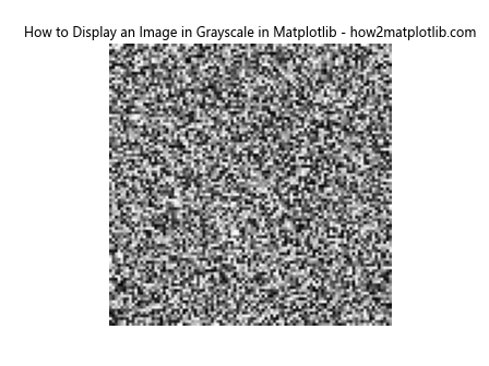
In this example, we create a random 100×100 grayscale image using NumPy and display it using Matplotlib’s imshow function. The cmap='gray' parameter specifies that we want to use a grayscale colormap for display.

Customizing Grayscale Display

When learning how to display an image in grayscale in Matplotlib, it’s important to understand the various customization options available. Let’s explore some of these options:

Adjusting Contrast and Brightness

import matplotlib.pyplot as plt
import numpy as np

# Create a sample grayscale image
grayscale_image = np.random.randint(0, 256, size=(100, 100))

# Adjust contrast and brightness
contrast = 1.5
brightness = 50
adjusted_image = np.clip(contrast * grayscale_image + brightness, 0, 255).astype(np.uint8)

# Display the adjusted grayscale image
plt.imshow(adjusted_image, cmap='gray')
plt.title('How to Display an Image in Grayscale in Matplotlib - Adjusted - how2matplotlib.com')
plt.axis('off')
plt.show()

Output:

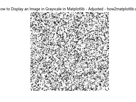
In this example, we demonstrate how to adjust the contrast and brightness of a grayscale image before displaying it. The np.clip function ensures that the pixel values remain within the valid range of 0-255.

Using Different Colormaps

While grayscale images are typically displayed using the ‘gray’ colormap, Matplotlib offers various other colormaps that can be used to represent grayscale data:

import matplotlib.pyplot as plt
import numpy as np

# Create a sample grayscale image
grayscale_image = np.random.randint(0, 256, size=(100, 100))

# Display the grayscale image with different colormaps
fig, axs = plt.subplots(2, 2, figsize=(10, 10))
cmaps = ['gray', 'viridis', 'plasma', 'inferno']

for ax, cmap in zip(axs.flat, cmaps):
    ax.imshow(grayscale_image, cmap=cmap)
    ax.set_title(f'Colormap: {cmap}')
    ax.axis('off')

plt.suptitle('How to Display an Image in Grayscale in Matplotlib - Colormaps - how2matplotlib.com')
plt.tight_layout()
plt.show()

Output:

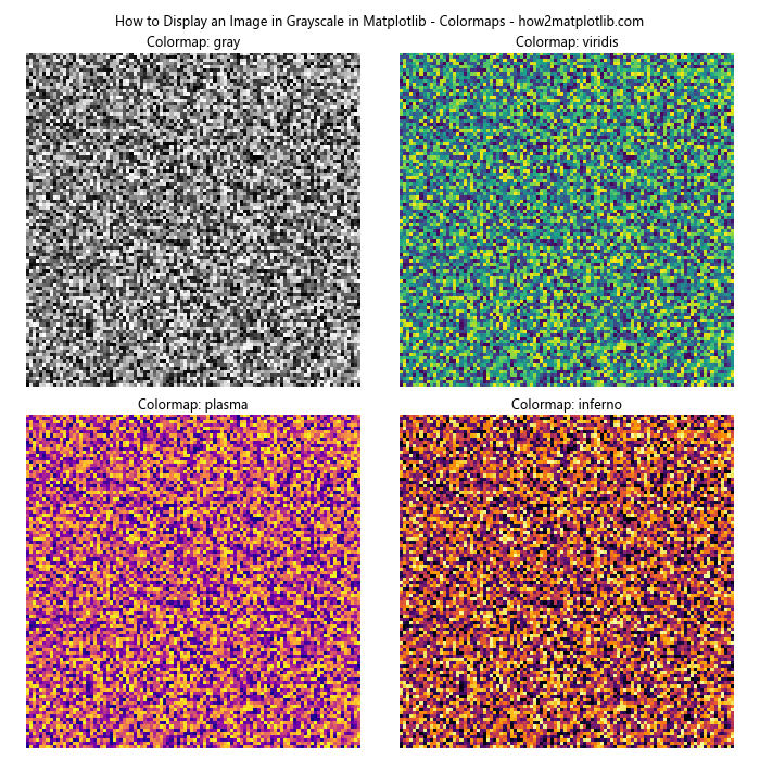
This example demonstrates how to display the same grayscale image using different colormaps. While not strictly grayscale, these alternative colormaps can sometimes reveal patterns or details that might be less visible in a traditional grayscale representation.

Adding Colorbar to Grayscale Images

When displaying grayscale images, it can be helpful to add a colorbar to show the mapping between pixel values and their visual representation:

import matplotlib.pyplot as plt
import numpy as np

# Create a sample grayscale image
grayscale_image = np.random.randint(0, 256, size=(100, 100))

# Display the grayscale image with a colorbar
fig, ax = plt.subplots(figsize=(8, 6))
im = ax.imshow(grayscale_image, cmap='gray')
ax.set_title('How to Display an Image in Grayscale in Matplotlib - with Colorbar - how2matplotlib.com')
ax.axis('off')

# Add colorbar
cbar = plt.colorbar(im)
cbar.set_label('Pixel Intensity')

plt.show()

Output:

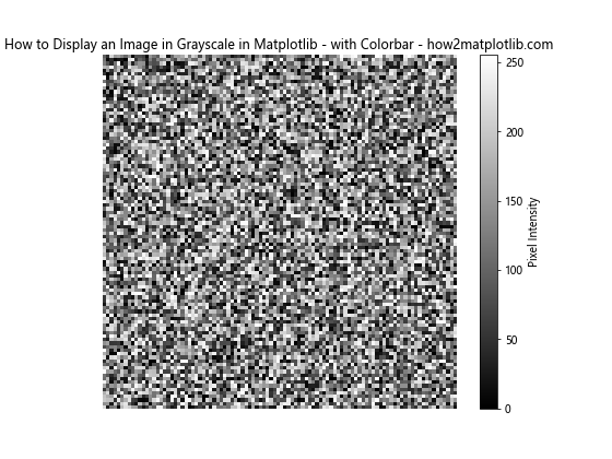
This example shows how to add a colorbar to a grayscale image display, which can be particularly useful for understanding the range and distribution of pixel intensities in the image.

Applying Filters to Grayscale Images

When working on how to display an image in grayscale in Matplotlib, you might want to apply various filters to enhance or modify the image before display:

import matplotlib.pyplot as plt
import numpy as np
from scipy import ndimage

# Create a sample grayscale image
grayscale_image = np.random.randint(0, 256, size=(100, 100))

# Apply Gaussian filter
filtered_image = ndimage.gaussian_filter(grayscale_image, sigma=2)

# Display original and filtered images
fig, (ax1, ax2) = plt.subplots(1, 2, figsize=(10, 5))

ax1.imshow(grayscale_image, cmap='gray')
ax1.set_title('Original Image')
ax1.axis('off')

ax2.imshow(filtered_image, cmap='gray')
ax2.set_title('Gaussian Filtered')
ax2.axis('off')

plt.suptitle('How to Display an Image in Grayscale in Matplotlib - Filtering - how2matplotlib.com')
plt.tight_layout()
plt.show()

Output:

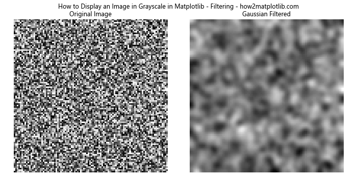
This example demonstrates how to apply a Gaussian filter to a grayscale image using SciPy’s ndimage module and display both the original and filtered images side by side.

Thresholding Grayscale Images

Thresholding is a common operation when working with grayscale images. Let’s explore how to display an image in grayscale in Matplotlib after applying a threshold:

import matplotlib.pyplot as plt
import numpy as np

# Create a sample grayscale image
grayscale_image = np.random.randint(0, 256, size=(100, 100))

# Apply threshold
threshold = 128
binary_image = (grayscale_image > threshold).astype(np.uint8) * 255

# Display original and thresholded images
fig, (ax1, ax2) = plt.subplots(1, 2, figsize=(10, 5))

ax1.imshow(grayscale_image, cmap='gray')
ax1.set_title('Original Image')
ax1.axis('off')

ax2.imshow(binary_image, cmap='gray')
ax2.set_title('Thresholded Image')
ax2.axis('off')

plt.suptitle('How to Display an Image in Grayscale in Matplotlib - Thresholding - how2matplotlib.com')
plt.tight_layout()
plt.show()

Output:

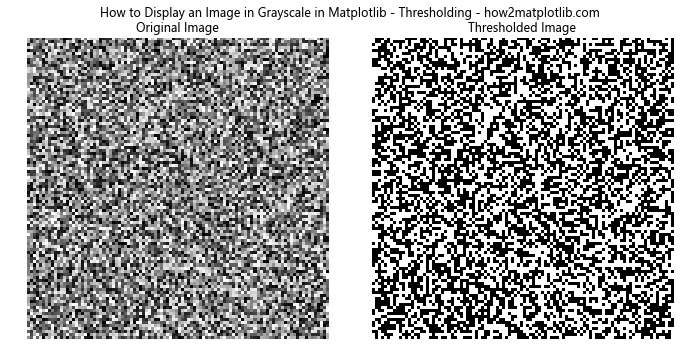
This example shows how to apply a simple threshold to a grayscale image, converting it to a binary image, and display both the original and thresholded images.

Displaying Grayscale Image Histograms

When working on how to display an image in grayscale in Matplotlib, it’s often useful to visualize the distribution of pixel intensities using a histogram:

import matplotlib.pyplot as plt
import numpy as np

# Create a sample grayscale image
grayscale_image = np.random.randint(0, 256, size=(100, 100))

# Display the grayscale image and its histogram
fig, (ax1, ax2) = plt.subplots(1, 2, figsize=(12, 5))

ax1.imshow(grayscale_image, cmap='gray')
ax1.set_title('Grayscale Image')
ax1.axis('off')

ax2.hist(grayscale_image.ravel(), bins=256, range=(0, 256))
ax2.set_title('Histogram')
ax2.set_xlabel('Pixel Intensity')
ax2.set_ylabel('Frequency')

plt.suptitle('How to Display an Image in Grayscale in Matplotlib - Histogram - how2matplotlib.com')
plt.tight_layout()
plt.show()

Output:

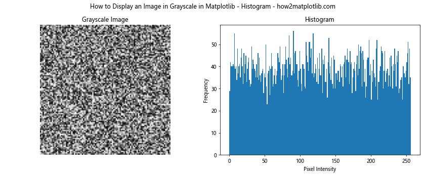
This example demonstrates how to display a grayscale image alongside its histogram, providing insights into the distribution of pixel intensities in the image.

Zooming and Panning Grayscale Images

When displaying large grayscale images, it’s often necessary to zoom in on specific regions. Let’s explore how to display an image in grayscale in Matplotlib with zooming and panning capabilities:

import matplotlib.pyplot as plt
import numpy as np
from matplotlib.widgets import RectangleSelector

# Create a large sample grayscale image
grayscale_image = np.random.randint(0, 256, size=(1000, 1000))

# Create the main plot
fig, (ax1, ax2) = plt.subplots(1, 2, figsize=(12, 6))
ax1.imshow(grayscale_image, cmap='gray')
ax1.set_title('Full Image')

# Initialize the zoomed view
zoomed = ax2.imshow(grayscale_image, cmap='gray')
ax2.set_title('Zoomed Region')

def onselect(eclick, erelease):
    x1, y1 = int(eclick.xdata), int(eclick.ydata)
    x2, y2 = int(erelease.xdata), int(erelease.ydata)
    zoomed.set_data(grayscale_image[y1:y2, x1:x2])
    ax2.set_xlim(0, x2-x1)
    ax2.set_ylim(y2-y1, 0)
    fig.canvas.draw_idle()

rs = RectangleSelector(ax1, onselect, interactive=True)

plt.suptitle('How to Display an Image in Grayscale in Matplotlib - Zooming - how2matplotlib.com')
plt.tight_layout()
plt.show()

Output:

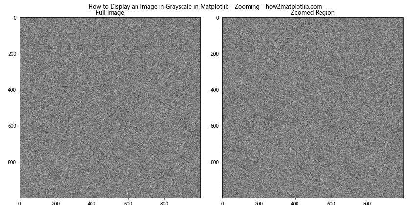
This example demonstrates how to implement a zooming feature using Matplotlib’s RectangleSelector widget. Users can select a region in the full image, and the zoomed view will update accordingly.

Displaying Grayscale Images with Annotations

When working on how to display an image in grayscale in Matplotlib, you may need to add annotations or highlights to specific regions of interest:

import matplotlib.pyplot as plt
import numpy as np

# Create a sample grayscale image
grayscale_image = np.random.randint(0, 256, size=(100, 100))

# Display the grayscale image with annotations
fig, ax = plt.subplots(figsize=(8, 8))
ax.imshow(grayscale_image, cmap='gray')

# Add a rectangle
rect = plt.Rectangle((20, 20), 30, 30, fill=False, edgecolor='red', linewidth=2)
ax.add_patch(rect)

# Add an arrow
ax.arrow(60, 60, 20, 20, head_width=5, head_length=5, fc='yellow', ec='yellow')

# Add text
ax.text(10, 90, 'Region of Interest', color='white', fontsize=12, bbox=dict(facecolor='black', alpha=0.5))

ax.set_title('How to Display an Image in Grayscale in Matplotlib - Annotations - how2matplotlib.com')
ax.axis('off')

plt.show()

Output:

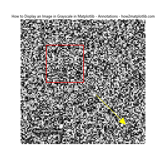
This example shows how to add various annotations to a grayscale image, including rectangles, arrows, and text. These annotations can be useful for highlighting specific features or regions of interest in the image.

Displaying Grayscale Images with Masked Regions

Sometimes when working on how to display an image in grayscale in Matplotlib, you may want to mask certain regions of the image:

import matplotlib.pyplot as plt
import numpy as np

# Create a sample grayscale image
grayscale_image = np.random.randint(0, 256, size=(100, 100))

# Create a mask
mask = np.zeros_like(grayscale_image, dtype=bool)
mask[30:70, 30:70] = True

# Apply the mask
masked_image = np.ma.array(grayscale_image, mask=mask)

# Display the masked grayscale image
fig, ax = plt.subplots(figsize=(8, 8))
ax.imshow(masked_image, cmap='gray')
ax.set_title('How to Display an Image in Grayscale in Matplotlib - Masked - how2matplotlib.com')
ax.axis('off')

plt.show()

Output:

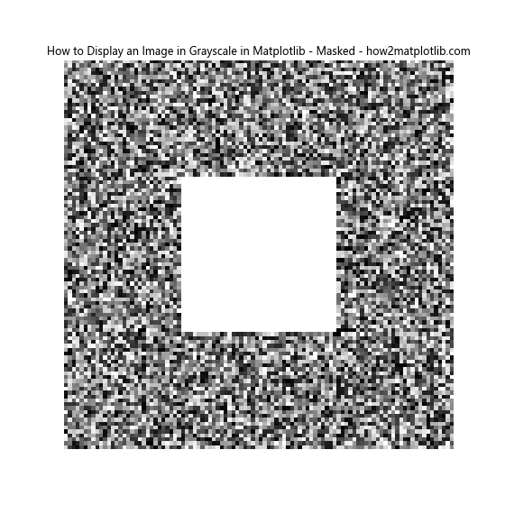
This example demonstrates how to create a mask and apply it to a grayscale image. The masked region will be displayed differently (typically transparent or with a different color) from the rest of the image.

Displaying Grayscale Images with Contours

Contour plots can be useful when working on how to display an image in grayscale in Matplotlib, especially for highlighting intensity levels:

import matplotlib.pyplot as plt
import numpy as np

# Create a sample grayscale image
x, y = np.meshgrid(np.linspace(-2, 2, 100), np.linspace(-2, 2, 100))
grayscale_image = np.exp(-(x**2 + y**2))

# Display the grayscale image with contours
fig, ax = plt.subplots(figsize=(8, 8))
im = ax.imshow(grayscale_image, cmap='gray')
contours = ax.contour(grayscale_image, colors='cyan', levels=5)
ax.clabel(contours, inline=True, fontsize=8)

ax.set_title('How to Display an Image in Grayscale in Matplotlib - Contours - how2matplotlib.com')
ax.axis('off')

plt.colorbar(im, label='Intensity')
plt.show()

Output:

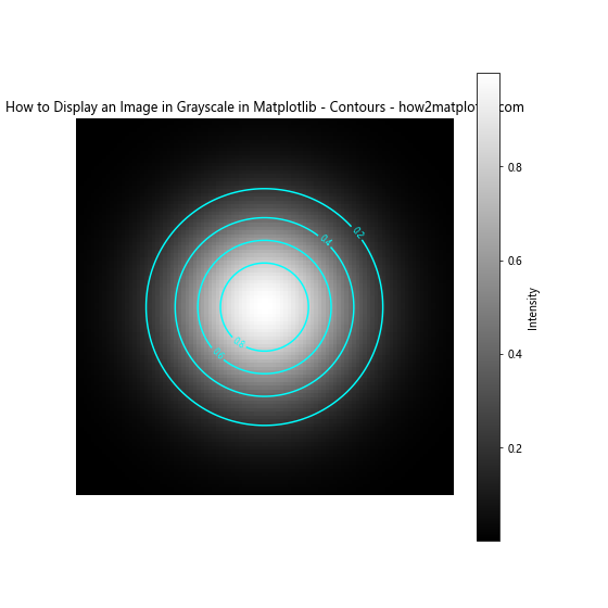
This example shows how to overlay contour lines on a grayscale image, which can be useful for visualizing intensity levels or gradients within the image.

Conclusion

In this comprehensive guide, we’ve explored various aspects of how to display an image in grayscale in Matplotlib. We’ve covered basic image display, loading and converting images, customizing display options, applying filters and transformations, and more advanced techniques like animation and annotation.

Mastering how to display an image in grayscale in Matplotlib is crucial for many data visualization and image processing tasks. The techniques we’ve discussed provide a solid foundation for working with grayscale images in Matplotlib, allowing you to effectively visualize and analyze image data in your projects.

Remember that Matplotlib offers a wide range of customization options and additional features beyond what we’ve covered here. As you continue to work with grayscale images, don’t hesitate to explore the Matplotlib documentation for more advanced techniques and options.

By understanding and applying these methods for how to display an image in grayscale in Matplotlib, you’ll be well-equipped to handle a variety of image visualization tasks in your data analysis and scientific computing projects.