How to Master Matplotlib Legend Location: A Comprehensive Guide

How to Master Matplotlib Legend Location: A Comprehensive Guide

Matplotlib legend location is a crucial aspect of data visualization that can significantly enhance the readability and interpretability of your plots. In this comprehensive guide, we’ll explore various techniques and best practices for optimizing the placement of legends in Matplotlib. From basic positioning to advanced customization, you’ll learn everything you need to know about matplotlib legend location to create professional-looking charts and graphs.

Understanding the Basics of Matplotlib Legend Location

Before diving into the specifics of matplotlib legend location, it’s essential to grasp the fundamental concepts. A legend in Matplotlib is a key that explains the meaning of different elements in your plot, such as lines, markers, or colors. The location of this legend can greatly impact the overall clarity and aesthetics of your visualization.

Let’s start with a simple example to illustrate the basic usage of matplotlib legend location:

import matplotlib.pyplot as plt

plt.figure(figsize=(8, 6))
plt.plot([1, 2, 3, 4], [1, 4, 2, 3], label='Line 1')
plt.plot([1, 2, 3, 4], [2, 3, 4, 1], label='Line 2')
plt.title('Basic Plot with Legend - how2matplotlib.com')
plt.legend(loc='best')
plt.show()

Output:

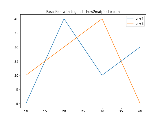
In this example, we create a simple plot with two lines and use plt.legend(loc='best') to automatically place the legend in the best location. The loc parameter is key to controlling matplotlib legend location.

Exploring Predefined Legend Locations in Matplotlib

Matplotlib offers several predefined locations for legend placement. These locations are specified using string values or numerical codes. Understanding these options is crucial for mastering matplotlib legend location.

Here’s an example showcasing different predefined legend locations:

import matplotlib.pyplot as plt

locations = ['best', 'upper right', 'upper left', 'lower left', 'lower right', 'right', 'center left', 'center right', 'lower center', 'upper center', 'center']

fig, axes = plt.subplots(4, 3, figsize=(15, 20))
axes = axes.flatten()

for i, loc in enumerate(locations):
    axes[i].plot([1, 2, 3, 4], [1, 4, 2, 3], label='Data')
    axes[i].set_title(f'Legend Location: {loc} - how2matplotlib.com')
    axes[i].legend(loc=loc)

plt.tight_layout()
plt.show()

Output:

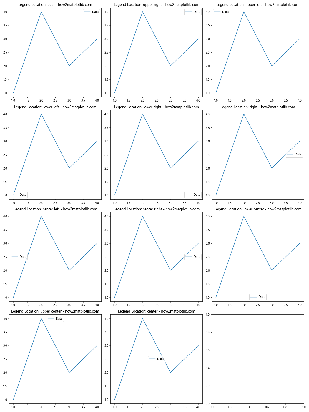
This code creates multiple subplots, each demonstrating a different predefined legend location. It’s an excellent way to visualize how matplotlib legend location affects the overall plot layout.

Fine-tuning Legend Position with Numerical Values

For more precise control over matplotlib legend location, you can use numerical values instead of string keywords. This method allows you to specify the exact coordinates of the legend within the plot area.

Here’s an example illustrating this technique:

import matplotlib.pyplot as plt

plt.figure(figsize=(8, 6))
plt.plot([1, 2, 3, 4], [1, 4, 2, 3], label='Data')
plt.title('Custom Legend Location - how2matplotlib.com')
plt.legend(loc=(0.7, 0.5))  # x, y coordinates (0-1 range)
plt.show()

Output:

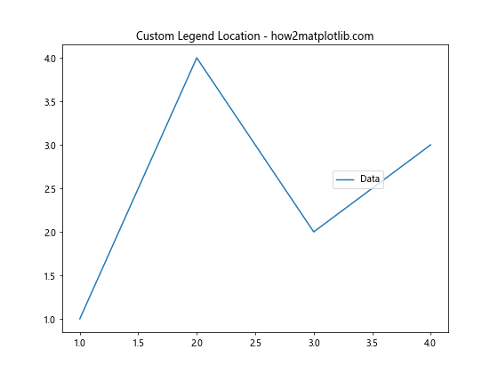
In this case, we set the legend location to (0.7, 0.5), which places it at 70% of the width and 50% of the height of the plot area. This level of precision in matplotlib legend location is particularly useful for complex plots where predefined locations may not suffice.

Adjusting Legend Box Alignment

Another aspect of matplotlib legend location is the alignment of the legend box itself. You can control how the legend box aligns with its specified location using the bbox_to_anchor parameter.

Let’s see an example:

import matplotlib.pyplot as plt

plt.figure(figsize=(8, 6))
plt.plot([1, 2, 3, 4], [1, 4, 2, 3], label='Data')
plt.title('Legend Box Alignment - how2matplotlib.com')
plt.legend(bbox_to_anchor=(1, 1), loc='upper left')
plt.tight_layout()
plt.show()

Output:

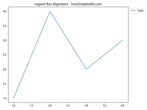
Here, we place the legend outside the plot area by setting bbox_to_anchor=(1, 1) and loc='upper left'. This combination positions the upper-left corner of the legend box at the top-right corner of the plot area.

Handling Multiple Legends in a Single Plot

Sometimes, you may need to include multiple legends in a single plot. This scenario requires special attention to matplotlib legend location to ensure clarity and avoid overlapping.

Here’s how you can manage multiple legends:

import matplotlib.pyplot as plt

fig, ax = plt.subplots(figsize=(8, 6))

line1, = ax.plot([1, 2, 3, 4], [1, 4, 2, 3], label='Data 1')
line2, = ax.plot([1, 2, 3, 4], [2, 3, 4, 1], label='Data 2')

first_legend = ax.legend(handles=[line1], loc='upper left')
ax.add_artist(first_legend)
ax.legend(handles=[line2], loc='lower right')

plt.title('Multiple Legends - how2matplotlib.com')
plt.show()

Output:

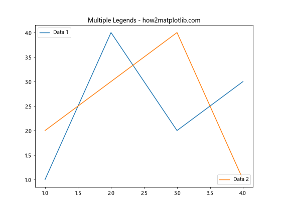
This example demonstrates how to create two separate legends and position them at different locations within the same plot. Mastering this technique is crucial for complex visualizations where matplotlib legend location plays a key role in data interpretation.

Customizing Legend Appearance for Better Readability

While location is important, the appearance of the legend itself can greatly affect its readability. Customizing the legend’s style can enhance the overall effectiveness of your matplotlib legend location strategy.

Let’s explore some customization options:

import matplotlib.pyplot as plt

plt.figure(figsize=(8, 6))
plt.plot([1, 2, 3, 4], [1, 4, 2, 3], label='Custom Legend')
plt.title('Customized Legend Appearance - how2matplotlib.com')
plt.legend(loc='best', frameon=False, fontsize=12, labelcolor='red', title='Legend Title', title_fontsize=14)
plt.show()

Output:

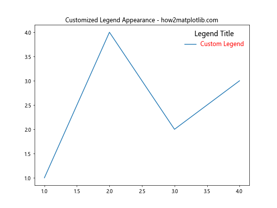
In this example, we’ve customized various aspects of the legend, including removing the frame, changing font sizes, and adding a title. These modifications can significantly improve the integration of the legend with your plot’s overall design.

Handling Legend Overflow with Multiple Columns

For plots with many data series, the legend can become quite large. In such cases, using multiple columns in the legend can help manage matplotlib legend location more effectively.

Here’s how to implement a multi-column legend:

import matplotlib.pyplot as plt

plt.figure(figsize=(10, 6))
for i in range(10):
    plt.plot([1, 2, 3, 4], [i]*4, label=f'Series {i+1}')
plt.title('Multi-Column Legend - how2matplotlib.com')
plt.legend(loc='lower center', ncol=5, bbox_to_anchor=(0.5, -0.2))
plt.tight_layout()
plt.show()

Output:

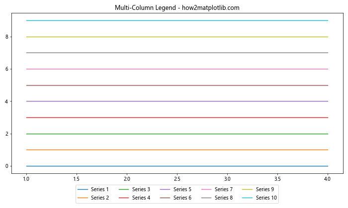
This code creates a plot with 10 data series and arranges the legend in 5 columns below the plot area. This approach is particularly useful when dealing with limited space and numerous legend entries.

Implementing Dynamic Legend Placement

In some cases, you might want to dynamically determine the best matplotlib legend location based on the data or other factors. While Matplotlib’s ‘best’ location often works well, you can create more sophisticated logic for placement.

Here’s an example of dynamic legend placement:

import matplotlib.pyplot as plt
import numpy as np

def find_clear_space(data):
    # Simple logic to find a clear space for the legend
    if np.mean(data[:len(data)//2]) > np.mean(data[len(data)//2:]):
        return 'lower right'
    else:
        return 'upper right'

plt.figure(figsize=(8, 6))
data = np.random.rand(100)
plt.plot(data, label='Random Data')
plt.title('Dynamic Legend Placement - how2matplotlib.com')
plt.legend(loc=find_clear_space(data))
plt.show()

Output:

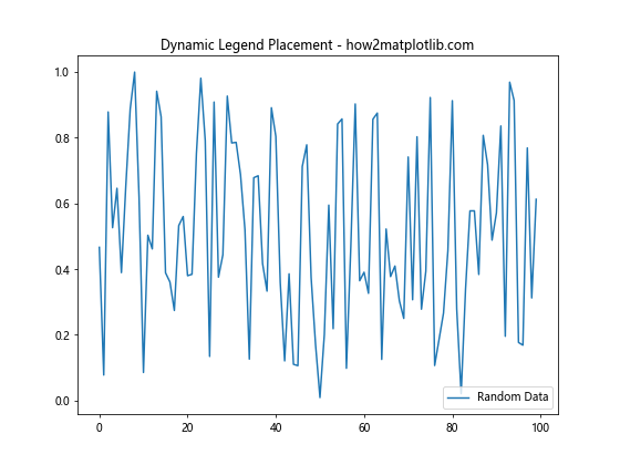
This script uses a simple function to determine whether the legend should be placed in the upper or lower right corner based on the data values. This dynamic approach to matplotlib legend location can be particularly useful for automated plotting systems.

Handling Legends in Subplots

When working with subplots, managing matplotlib legend location becomes more challenging. You need to consider the layout of multiple plots and how legends interact with each other.

Here’s an example of handling legends in a subplot layout:

import matplotlib.pyplot as plt

fig, (ax1, ax2) = plt.subplots(1, 2, figsize=(12, 5))

ax1.plot([1, 2, 3, 4], [1, 4, 2, 3], label='Data 1')
ax1.set_title('Subplot 1 - how2matplotlib.com')
ax1.legend(loc='best')

ax2.plot([1, 2, 3, 4], [2, 3, 4, 1], label='Data 2')
ax2.set_title('Subplot 2 - how2matplotlib.com')
ax2.legend(loc='best')

plt.tight_layout()
plt.show()

Output:

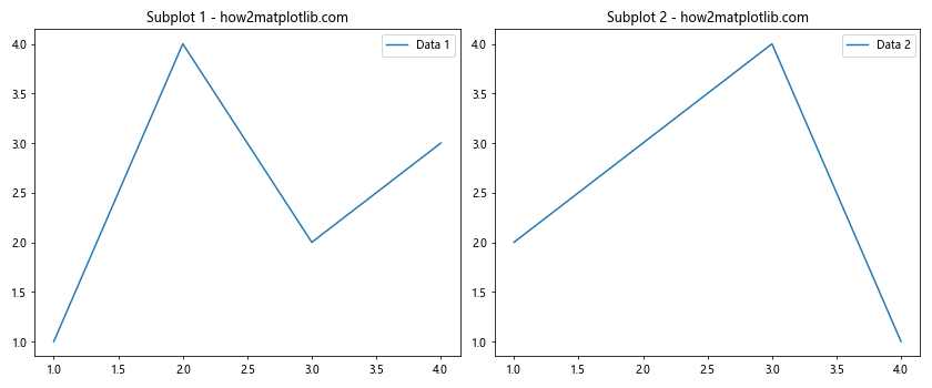
This code creates two subplots, each with its own legend. The ‘best’ location is used for each subplot, allowing Matplotlib to determine the optimal placement within each individual plot area.

Creating a Shared Legend for Multiple Subplots

In some cases, you might want to create a single, shared legend for multiple subplots. This approach can save space and provide a cleaner overall layout.

Here’s how to implement a shared legend:

import matplotlib.pyplot as plt

fig, (ax1, ax2) = plt.subplots(1, 2, figsize=(12, 5))

line1, = ax1.plot([1, 2, 3, 4], [1, 4, 2, 3], label='Data 1')
ax1.set_title('Subplot 1 - how2matplotlib.com')

line2, = ax2.plot([1, 2, 3, 4], [2, 3, 4, 1], label='Data 2')
ax2.set_title('Subplot 2 - how2matplotlib.com')

fig.legend(handles=[line1, line2], loc='lower center', bbox_to_anchor=(0.5, -0.05), ncol=2)

plt.tight_layout()
plt.show()

Output:

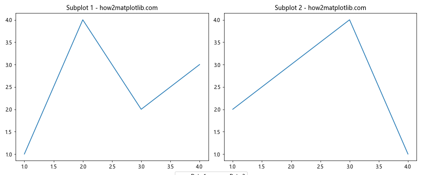
This example creates a single legend for both subplots, positioned below them. This technique is particularly useful when dealing with related data across multiple subplots.

Optimizing Legend Location for Different Plot Types

Different types of plots may require different approaches to matplotlib legend location. For instance, the optimal legend placement for a scatter plot might differ from that of a bar chart.

Let’s look at an example with a pie chart:

import matplotlib.pyplot as plt

plt.figure(figsize=(8, 8))
sizes = [15, 30, 45, 10]
labels = ['A', 'B', 'C', 'D']
plt.pie(sizes, labels=labels, autopct='%1.1f%%', startangle=90)
plt.title('Pie Chart with Legend - how2matplotlib.com')
plt.legend(title='Categories', loc='center left', bbox_to_anchor=(1, 0.5))
plt.axis('equal')
plt.tight_layout()
plt.show()

Output:

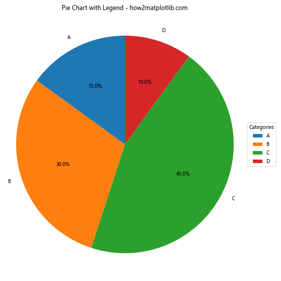
In this pie chart example, we place the legend to the right of the chart. This arrangement works well for circular plots where legend entries correspond to pie slices.

Handling Legend Location in 3D Plots

When working with 3D plots in Matplotlib, legend location requires special consideration. The 3D space introduces new challenges and opportunities for legend placement.

Here’s an example of a 3D plot with a legend:

import matplotlib.pyplot as plt
from mpl_toolkits.mplot3d import Axes3D
import numpy as np

fig = plt.figure(figsize=(8, 6))
ax = fig.add_subplot(111, projection='3d')

x = np.random.rand(100)
y = np.random.rand(100)
z = np.random.rand(100)

scatter = ax.scatter(x, y, z, c=z, cmap='viridis', label='3D Data')
ax.set_xlabel('X axis')
ax.set_ylabel('Y axis')
ax.set_zlabel('Z axis')
ax.set_title('3D Plot with Legend - how2matplotlib.com')

ax.legend()
plt.colorbar(scatter)
plt.show()

Output:

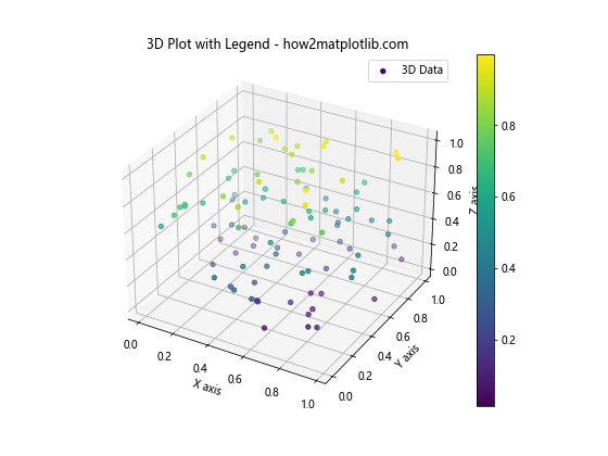
In this 3D scatter plot, we let Matplotlib automatically determine the best legend location. For 3D plots, it’s often best to use automatic placement or position the legend outside the plot area to avoid obscuring the data.

Using Legend Location to Highlight Key Information

Strategic use of matplotlib legend location can help highlight key information in your plots. By placing the legend near important data points or trends, you can draw the viewer’s attention to crucial aspects of your visualization.

Consider this example:

import matplotlib.pyplot as plt
import numpy as np

plt.figure(figsize=(10, 6))
x = np.linspace(0, 10, 100)
y1 = np.sin(x)
y2 = np.cos(x)

plt.plot(x, y1, label='sin(x)')
plt.plot(x, y2, label='cos(x)')
plt.title('Highlighting Intersection - how2matplotlib.com')

intersection_x = np.pi / 4
plt.plot(intersection_x, np.sin(intersection_x), 'ro')

plt.legend(loc='center', bbox_to_anchor=(0.5, 0.3))
plt.annotate('Intersection', xy=(intersection_x, np.sin(intersection_x)), xytext=(4, 0.5),
             arrowprops=dict(facecolor='black', shrink=0.05))

plt.show()

Output:

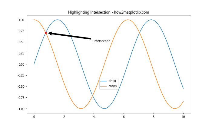
In this plot, we’ve positioned the legend near the intersection point of the sine and cosine curves, drawing attention to this key feature of the graph.

Incorporating Interactive Legend Placement

For interactive applications, allowing users to dynamically adjust the matplotlib legend location can greatly enhance the user experience. While this typically requires more advanced tools like Jupyter widgets or web frameworks, we can simulate the concept with a simple example:

import matplotlib.pyplot as plt
from matplotlib.widgets import RadioButtons

fig, ax = plt.subplots(figsize=(8, 6))
ax.plot([1, 2, 3, 4], [1, 4, 2, 3], label='Data')
ax.set_title('Interactive Legend Placement - how2matplotlib.com')

legend = ax.legend(loc='best')

rax = plt.axes([0.01, 0.7, 0.15, 0.15])
radio = RadioButtons(rax, ('best', 'upper right', 'upper left', 'lower left'))

def change_legend_loc(label):
    legend.set_visible(False)
    ax.legend(loc=label)
    plt.draw()

radio.on_clicked(change_legend_loc)

plt.show()

Output:

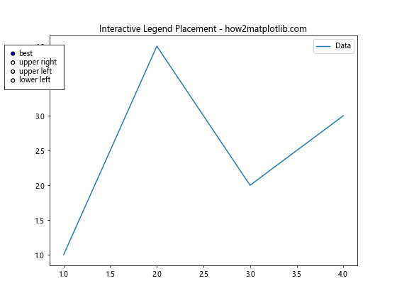
This example creates a plot with radio buttons that allow changing the legend location interactively. While this specific implementation works in certain environments, it illustrates the concept of dynamic legend placement.

Balancing Legend Location with Data Visibility

One of the key challenges in matplotlib legend location is ensuring that the legend doesn’t obscure important data points. This is particularly crucial in dense plots or when working with multiple data series.

Here’s an approach to address this issue:

import matplotlib.pyplot as plt
import numpy as np

plt.figure(figsize=(10, 6))

# Generate some sample data
x = np.linspace(0, 10, 100)
for i in range(5):
    y = np.sin(x + i*0.5) + np.random.normal(0, 0.1, 100)
    plt.plot(x, y, label=f'Series {i+1}')

plt.title('Balancing Legend and Data Visibility - how2matplotlib.com')

# Place legend outside the plot area
plt.legend(bbox_to_anchor=(1.05, 1), loc='upper left')

plt.tight_layout()
plt.show()

Output:

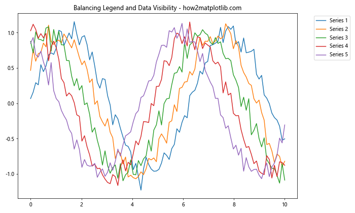
In this example, we place the legend outside the plot area to ensure it doesn’t overlap with any of the multiple data series. This approach is particularly useful for plots with many overlapping lines or points.

Leveraging Legend Location in Comparative Plots

When creating plots that compare multiple datasets, strategic placement of legends can significantly enhance the clarity of the comparison. Let’s look at an example using a box plot:

import matplotlib.pyplot as plt
import numpy as np

plt.figure(figsize=(10, 6))

data = [np.random.normal(0, std, 100) for std in range(1, 5)]
labels = ['A', 'B', 'C', 'D']

box_plot = plt.boxplot(data, labels=labels, patch_artist=True)

colors = ['lightblue', 'lightgreen', 'lightpink', 'lightyellow']
for patch, color in zip(box_plot['boxes'], colors):
    patch.set_facecolor(color)

plt.title('Comparative Box Plot with Legend - how2matplotlib.com')
plt.legend(box_plot['boxes'], labels, title='Groups', loc='upper left', bbox_to_anchor=(1, 1))

plt.tight_layout()
plt.show()

Output:

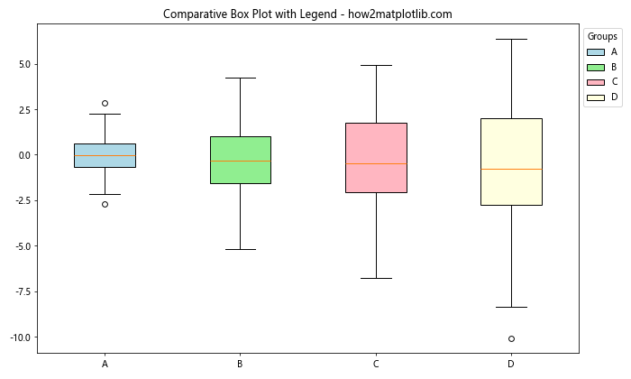
In this comparative box plot, we place the legend to the right of the plot, clearly associating each box with its corresponding group label. This arrangement facilitates easy comparison between the different datasets.

Optimizing Legend Location for Publication-Quality Figures

When preparing figures for publication, paying close attention to matplotlib legend location can make a significant difference in the professional appearance of your plots. Here’s an example of a publication-quality figure with carefully placed legends:

import matplotlib.pyplot as plt
import numpy as np

plt.figure(figsize=(10, 8))

x = np.linspace(0, 10, 100)
y1 = np.sin(x)
y2 = np.cos(x)
y3 = np.tan(x)

plt.plot(x, y1, 'b-', label='sin(x)')
plt.plot(x, y2, 'r--', label='cos(x)')
plt.plot(x, y3, 'g:', label='tan(x)')

plt.title('Trigonometric Functions - how2matplotlib.com', fontsize=16)
plt.xlabel('x', fontsize=14)
plt.ylabel('y', fontsize=14)

plt.legend(loc='upper center', bbox_to_anchor=(0.5, -0.05), ncol=3, fontsize=12)

plt.grid(True, linestyle='--', alpha=0.7)
plt.tight_layout()
plt.show()

Output:

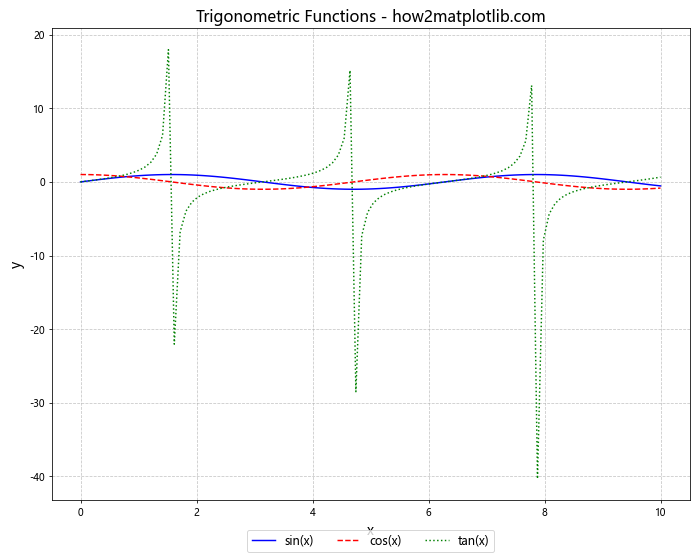
This example demonstrates a clean, professional-looking plot with the legend placed below the graph. The use of multiple columns in the legend and careful positioning ensures that it complements the plot without detracting from the data presentation.

Conclusion: Mastering Matplotlib Legend Location

Throughout this comprehensive guide, we’ve explored various aspects of matplotlib legend location, from basic positioning to advanced techniques for complex plots. We’ve seen how the right legend placement can significantly enhance the clarity and effectiveness of data visualizations.

Key takeaways include:

1. Understanding the basic loc parameter and predefined locations.
2. Using numerical values for precise legend positioning.
3. Leveraging bbox_to_anchor for flexible legend placement.
4. Handling multiple legends and legends in subplots.
5. Customizing legend appearance for better readability.
6. Adapting legend location for different plot types and figure sizes.
7. Balancing legend placement with data visibility.
8. Optimizing legend location for publication-quality figures.

By mastering these techniques, you can ensure that your matplotlib legends not only provide essential information but also contribute to the overall aesthetic and clarity of your visualizations. Remember, the ideal matplotlib legend location often depends on the specific data and the story you’re trying to tell with your plot. Experiment with different approaches and always consider your audience and the context in which your visualizations will be viewed.

As you continue to work with Matplotlib, keep exploring new ways to refine your legend placements. The flexibility and power of Matplotlib’s legend system offer endless possibilities for creating informative and visually appealing data visualizations.