How to Use Matplotlib.figure.Figure.set_constrained_layout_pads() in Python for Optimal Plot Layout
Matplotlib.figure.Figure.set_constrained_layout_pads() in Python is a powerful method that allows you to fine-tune the padding around subplots when using constrained layout in Matplotlib. This function is particularly useful when you need to adjust the spacing between subplots and the figure edges to create visually appealing and well-organized plots. In this comprehensive guide, we’ll explore the various aspects of Matplotlib.figure.Figure.set_constrained_layout_pads() and provide numerous examples to help you master this essential tool for plot customization.
Understanding Matplotlib.figure.Figure.set_constrained_layout_pads()
Matplotlib.figure.Figure.set_constrained_layout_pads() is a method that belongs to the Figure class in Matplotlib. It is used to set the padding parameters for constrained layout, which is an automatic layout mechanism that adjusts the positions of plot elements to prevent overlapping and ensure proper spacing. The method takes four parameters: w_pad, h_pad, wspace, and hspace, which control the padding and spacing in different directions.
Let’s break down the parameters of Matplotlib.figure.Figure.set_constrained_layout_pads():
- w_pad: Controls the padding on the left and right sides of the figure.
- h_pad: Controls the padding on the top and bottom of the figure.
- wspace: Controls the horizontal space between subplots.
- hspace: Controls the vertical space between subplots.
Now, let’s dive into some examples to see how we can use Matplotlib.figure.Figure.set_constrained_layout_pads() in practice.
Basic Usage of Matplotlib.figure.Figure.set_constrained_layout_pads()
To start, let’s create a simple example that demonstrates the basic usage of Matplotlib.figure.Figure.set_constrained_layout_pads():
import matplotlib.pyplot as plt
import numpy as np

# Create a figure with constrained layout
fig, axs = plt.subplots(2, 2, constrained_layout=True, figsize=(10, 8))

# Generate some sample data
x = np.linspace(0, 10, 100)
y1 = np.sin(x)
y2 = np.cos(x)
y3 = np.tan(x)
y4 = np.exp(-x/5)

# Plot the data
axs[0, 0].plot(x, y1, label='sin(x)')
axs[0, 1].plot(x, y2, label='cos(x)')
axs[1, 0].plot(x, y3, label='tan(x)')
axs[1, 1].plot(x, y4, label='exp(-x/5)')

# Add labels and titles
for ax in axs.flat:
    ax.set_xlabel('x')
    ax.set_ylabel('y')
    ax.legend()
    ax.set_title('Plot from how2matplotlib.com')

# Set constrained layout pads
fig.set_constrained_layout_pads(w_pad=0.1, h_pad=0.1, wspace=0.1, hspace=0.1)

plt.show()
Output:
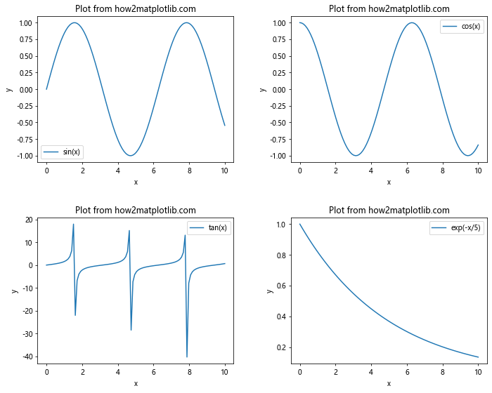
In this example, we create a 2×2 grid of subplots using constrained layout. We then use Matplotlib.figure.Figure.set_constrained_layout_pads() to set the padding and spacing between the subplots. The w_pad and h_pad values control the padding around the entire figure, while wspace and hspace control the spacing between individual subplots.
Adjusting Padding for Different Plot Types
Matplotlib.figure.Figure.set_constrained_layout_pads() can be particularly useful when working with different types of plots that may require varying amounts of space. Let’s explore how to use this method with bar plots and scatter plots:
import matplotlib.pyplot as plt
import numpy as np

# Create a figure with constrained layout
fig, (ax1, ax2) = plt.subplots(1, 2, constrained_layout=True, figsize=(12, 5))

# Generate data for bar plot
categories = ['A', 'B', 'C', 'D', 'E']
values = [3, 7, 2, 5, 8]

# Create bar plot
ax1.bar(categories, values)
ax1.set_title('Bar Plot from how2matplotlib.com')
ax1.set_xlabel('Categories')
ax1.set_ylabel('Values')

# Generate data for scatter plot
x = np.random.rand(50)
y = np.random.rand(50)
colors = np.random.rand(50)
sizes = 1000 * np.random.rand(50)

# Create scatter plot
scatter = ax2.scatter(x, y, c=colors, s=sizes, alpha=0.5)
ax2.set_title('Scatter Plot from how2matplotlib.com')
ax2.set_xlabel('X')
ax2.set_ylabel('Y')

# Add colorbar
plt.colorbar(scatter, ax=ax2, label='Color')

# Set constrained layout pads
fig.set_constrained_layout_pads(w_pad=0.2, h_pad=0.2, wspace=0.3, hspace=0.2)

plt.show()
Output:
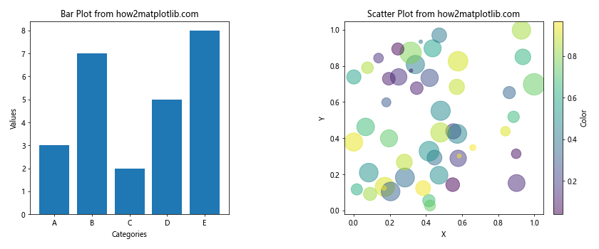
In this example, we create a figure with two subplots: a bar plot and a scatter plot. We use Matplotlib.figure.Figure.set_constrained_layout_pads() to adjust the padding and spacing to accommodate the different plot types and the colorbar.
Fine-tuning Padding for Complex Layouts
When working with more complex layouts, Matplotlib.figure.Figure.set_constrained_layout_pads() becomes even more valuable. Let’s create an example with a mixed layout of subplots:
import matplotlib.pyplot as plt
import numpy as np

# Create a figure with constrained layout
fig = plt.figure(constrained_layout=True, figsize=(12, 8))

# Create a complex grid of subplots
gs = fig.add_gridspec(3, 3)
ax1 = fig.add_subplot(gs[0, :])
ax2 = fig.add_subplot(gs[1, :-1])
ax3 = fig.add_subplot(gs[1:, -1])
ax4 = fig.add_subplot(gs[-1, 0])
ax5 = fig.add_subplot(gs[-1, -2])

# Generate some sample data
x = np.linspace(0, 10, 100)
y1 = np.sin(x)
y2 = np.cos(x)
y3 = np.tan(x)
y4 = np.exp(-x/5)
y5 = x**2

# Plot the data
ax1.plot(x, y1, label='sin(x)')
ax2.plot(x, y2, label='cos(x)')
ax3.plot(x, y3, label='tan(x)')
ax4.plot(x, y4, label='exp(-x/5)')
ax5.plot(x, y5, label='x^2')

# Add labels and titles
for ax in [ax1, ax2, ax3, ax4, ax5]:
    ax.set_xlabel('x')
    ax.set_ylabel('y')
    ax.legend()
    ax.set_title('Plot from how2matplotlib.com')

# Set constrained layout pads
fig.set_constrained_layout_pads(w_pad=0.2, h_pad=0.3, wspace=0.1, hspace=0.2)

plt.show()
Output:
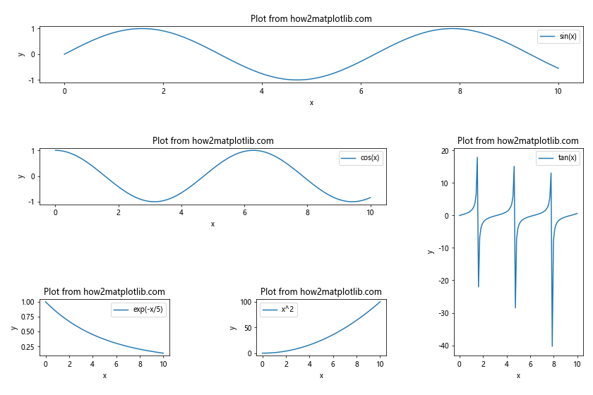
In this example, we create a more complex layout with subplots of different sizes and positions. Matplotlib.figure.Figure.set_constrained_layout_pads() helps us adjust the padding and spacing to ensure that all subplots are properly arranged and visible.
Optimizing Padding for Different Figure Sizes
When working with different figure sizes, you may need to adjust the padding parameters accordingly. Let’s explore how to use Matplotlib.figure.Figure.set_constrained_layout_pads() with various figure sizes:
import matplotlib.pyplot as plt
import numpy as np

def create_plot(figsize, w_pad, h_pad, wspace, hspace):
    fig, axs = plt.subplots(2, 2, constrained_layout=True, figsize=figsize)

    x = np.linspace(0, 10, 100)
    y1 = np.sin(x)
    y2 = np.cos(x)
    y3 = np.tan(x)
    y4 = np.exp(-x/5)

    axs[0, 0].plot(x, y1, label='sin(x)')
    axs[0, 1].plot(x, y2, label='cos(x)')
    axs[1, 0].plot(x, y3, label='tan(x)')
    axs[1, 1].plot(x, y4, label='exp(-x/5)')

    for ax in axs.flat:
        ax.set_xlabel('x')
        ax.set_ylabel('y')
        ax.legend()
        ax.set_title('Plot from how2matplotlib.com')

    fig.set_constrained_layout_pads(w_pad=w_pad, h_pad=h_pad, wspace=wspace, hspace=hspace)

    plt.show()

# Small figure
create_plot((6, 4), w_pad=0.1, h_pad=0.1, wspace=0.2, hspace=0.2)

# Medium figure
create_plot((10, 8), w_pad=0.2, h_pad=0.2, wspace=0.3, hspace=0.3)

# Large figure
create_plot((16, 12), w_pad=0.3, h_pad=0.3, wspace=0.4, hspace=0.4)
In this example, we create a function that generates plots with different figure sizes and padding parameters. We then call this function three times with varying figure sizes to demonstrate how Matplotlib.figure.Figure.set_constrained_layout_pads() can be used to optimize the layout for different figure dimensions.
Handling Tight Layouts with Matplotlib.figure.Figure.set_constrained_layout_pads()
Sometimes, you may need to create plots with very tight layouts, where space is at a premium. Matplotlib.figure.Figure.set_constrained_layout_pads() can help you achieve this while still maintaining readability:
import matplotlib.pyplot as plt
import numpy as np

# Create a figure with constrained layout
fig, axs = plt.subplots(3, 3, constrained_layout=True, figsize=(10, 10))

# Generate some sample data
x = np.linspace(0, 10, 100)
y = [np.sin(x), np.cos(x), np.tan(x), np.exp(-x/5), x**2, np.log(x+1), np.sqrt(x), x**3, 1/x]

# Plot the data
for i, ax in enumerate(axs.flat):
    ax.plot(x, y[i])
    ax.set_title(f'Plot {i+1} from how2matplotlib.com', fontsize=8)
    ax.tick_params(axis='both', which='major', labelsize=6)
    ax.tick_params(axis='both', which='minor', labelsize=4)

# Set very tight constrained layout pads
fig.set_constrained_layout_pads(w_pad=0.01, h_pad=0.01, wspace=0.05, hspace=0.05)

plt.show()
Output:
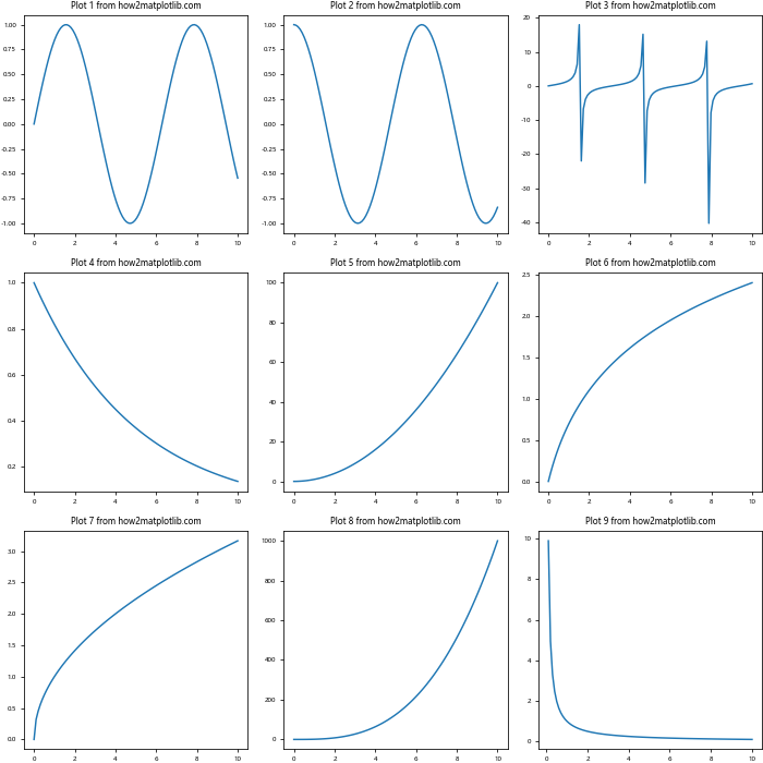
In this example, we create a 3×3 grid of subplots with very tight spacing. By using small values for the padding parameters in Matplotlib.figure.Figure.set_constrained_layout_pads(), we can create a compact layout while still maintaining the visibility of all plot elements.
Combining Matplotlib.figure.Figure.set_constrained_layout_pads() with Subplots of Different Sizes
Matplotlib.figure.Figure.set_constrained_layout_pads() can be particularly useful when working with subplots of different sizes. Let’s explore an example that demonstrates this:
import matplotlib.pyplot as plt
import numpy as np

# Create a figure with constrained layout
fig = plt.figure(constrained_layout=True, figsize=(12, 8))

# Create a grid of subplots with different sizes
gs = fig.add_gridspec(3, 3)
ax1 = fig.add_subplot(gs[0, :])
ax2 = fig.add_subplot(gs[1:, 0])
ax3 = fig.add_subplot(gs[1:, 1:])

# Generate some sample data
x = np.linspace(0, 10, 100)
y1 = np.sin(x)
y2 = np.cos(x)
y3 = np.tan(x)

# Plot the data
ax1.plot(x, y1, label='sin(x)')
ax2.plot(x, y2, label='cos(x)')
ax3.plot(x, y3, label='tan(x)')

# Add labels and titles
for ax, title in zip([ax1, ax2, ax3], ['Sin', 'Cos', 'Tan']):
    ax.set_xlabel('x')
    ax.set_ylabel('y')
    ax.legend()
    ax.set_title(f'{title} Plot from how2matplotlib.com')

# Set constrained layout pads
fig.set_constrained_layout_pads(w_pad=0.2, h_pad=0.3, wspace=0.1, hspace=0.2)

plt.show()
Output:
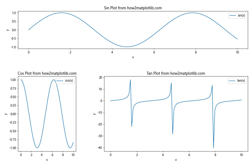
In this example, we create a layout with subplots of different sizes: one spanning the entire top row, one occupying the left half of the remaining space, and one taking up the right half of the remaining space. Matplotlib.figure.Figure.set_constrained_layout_pads() helps us adjust the padding and spacing to ensure that all subplots are properly arranged and visible, despite their different sizes.
Using Matplotlib.figure.Figure.set_constrained_layout_pads() with Colorbars and Legends
When working with plots that include colorbars and legends, Matplotlib.figure.Figure.set_constrained_layout_pads() can help you fine-tune the layout to accommodate these additional elements. Let’s look at an example:
import matplotlib.pyplot as plt
import numpy as np

# Create a figure with constrained layout
fig, (ax1, ax2) = plt.subplots(1, 2, constrained_layout=True, figsize=(12, 5))

# Generate data for heatmap
data1 = np.random.rand(10, 10)

# Create heatmap
im1 = ax1.imshow(data1, cmap='viridis')
ax1.set_title('Heatmap from how2matplotlib.com')
fig.colorbar(im1, ax=ax1, label='Value')

# Generate data for scatter plot
x = np.random.rand(50)
y = np.random.rand(50)
colors = np.random.rand(50)
sizes = 1000 * np.random.rand(50)

# Create scatter plot
scatter = ax2.scatter(x, y, c=colors, s=sizes, alpha=0.5)
ax2.set_title('Scatter Plot from how2matplotlib.com')
ax2.set_xlabel('X')
ax2.set_ylabel('Y')
fig.colorbar(scatter, ax=ax2, label='Color')

# Add a legend to the scatter plot
legend_elements = [plt.scatter([], [], s=100, label='Small'),
                   plt.scatter([], [], s=500, label='Medium'),
                   plt.scatter([], [], s=1000, label='Large')]
ax2.legend(handles=legend_elements, title='Size', loc='upper left')

# Set constrained layout pads
fig.set_constrained_layout_pads(w_pad=0.2, h_pad=0.2, wspace=0.3, hspace=0.2)

plt.show()
Output:
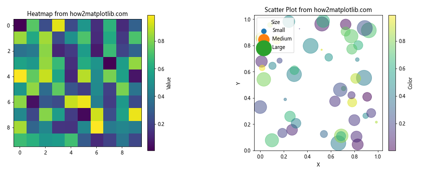
In this example, we create two subplots: a heatmap with a colorbar and a scatter plot with both a colorbar and a legend. By using Matplotlib.figure.Figure.set_constrained_layout_pads(), we can adjust the padding and spacing to accommodate these additional elements while maintaining a clean and readable layout.
Adapting Matplotlib.figure.Figure.set_constrained_layout_pads() for Different Aspect Ratios
When working with plots that have different aspect ratios, you may need to adjust the padding parameters accordingly. Let’s explore how to use Matplotlib.figure.Figure.set_constrained_layout_pads() with various aspect ratios:
import matplotlib.pyplot as plt
import numpy as np

def create_plot(aspect_ratio, w_pad, h_pad, wspace, hspace):
    fig, axs = plt.subplots(2, 2, constrained_layout=True, figsize=(10 * aspect_ratio, 10))

    x = np.linspace(0, 10, 100)
    y1 = np.sin(x)
    y2 = np.cos(x)
    y3 = np.tan(x)
    y4 = np.exp(-x/5)

    axs[0, 0].plot(x, y1, label='sin(x)')
    axs[0, 1].plot(x, y2, label='cos(x)')
    axs[1, 0].plot(x, y3, label='tan(x)')
    axs[1, 1].plot(x, y4, label='exp(-x/5)')

    for ax in axs.flat:
        ax.set_xlabel('x')
        ax.set_ylabel('y')
        ax.legend()
        ax.set_title(f'Plot from how2matplotlib.com (Aspect Ratio: {aspect_ratio})')

    fig.set_constrained_layout_pads(w_pad=w_pad, h_pad=h_pad, wspace=wspace, hspace=hspace)

    plt.show()

# Wide aspect ratio
create_plot(1.5, w_pad=0.2, h_pad=0.1, wspace=0.3, hspace=0.2)

# Square aspect ratio
create_plot(1.0, w_pad=0.2, h_pad=0.2, wspace=0.2, hspace=0.2)

# Tall aspect ratio
create_plot(0.75, w_pad=0.1, h_pad=0.2, wspace=0.2, hspace=0.3)
In this example, we create a function that generates plots with different aspect ratios and padding parameters. We then call this function three times with varying aspect ratios to demonstrate how Matplotlib.figure.Figure.set_constrained_layout_pads() can be used to optimize the layout for different figure dimensions.
Using Matplotlib.figure.Figure.set_constrained_layout_pads() with Annotations and Text
When adding annotations and text to your plots, you may need to adjust the padding to ensure that all elements are visible and properly positioned. Let’s look at an example that demonstrates how to use Matplotlib.figure.Figure.set_constrained_layout_pads() with annotations and text:
import matplotlib.pyplot as plt
import numpy as np

# Create a figure with constrained layout
fig, axs = plt.subplots(2, 2, constrained_layout=True, figsize=(12, 10))

# Generate some sample data
x = np.linspace(0, 10, 100)
y1 = np.sin(x)
y2 = np.cos(x)
y3 = np.tan(x)
y4 = np.exp(-x/5)

# Plot the data and add annotations
axs[0, 0].plot(x, y1, label='sin(x)')
axs[0, 0].annotate('Peak', xy=(np.pi/2, 1), xytext=(np.pi/2 + 1, 1.2),
                   arrowprops=dict(facecolor='black', shrink=0.05))

axs[0, 1].plot(x, y2, label='cos(x)')
axs[0, 1].text(5, 0.5, 'Cosine Wave', fontsize=12, bbox=dict(facecolor='white', alpha=0.5))

axs[1, 0].plot(x, y3, label='tan(x)')
axs[1, 0].annotate('Asymptote', xy=(np.pi/2, 10), xytext=(np.pi/2 + 1, 8),
                   arrowprops=dict(facecolor='black', shrink=0.05))

axs[1, 1].plot(x, y4, label='exp(-x/5)')
axs[1, 1].text(2, 0.8, 'Exponential Decay', fontsize=12, bbox=dict(facecolor='white', alpha=0.5))

# Add labels and titles
for ax in axs.flat:
    ax.set_xlabel('x')
    ax.set_ylabel('y')
    ax.legend()
    ax.set_title('Plot from how2matplotlib.com')

# Set constrained layout pads
fig.set_constrained_layout_pads(w_pad=0.3, h_pad=0.3, wspace=0.4, hspace=0.4)

plt.show()
Output:
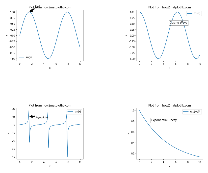
In this example, we create a 2×2 grid of subplots and add various annotations and text elements to each plot. By using Matplotlib.figure.Figure.set_constrained_layout_pads(), we can adjust the padding and spacing to ensure that all annotations and text are visible and do not overlap with other plot elements.
Combining Matplotlib.figure.Figure.set_constrained_layout_pads() with Subplots of Different Types
When working with a mix of different plot types, you may need to adjust the padding to accommodate their varying sizes and shapes. Let’s explore an example that combines different types of plots:
import matplotlib.pyplot as plt
import numpy as np

# Create a figure with constrained layout
fig = plt.figure(constrained_layout=True, figsize=(12, 10))

# Create a grid of subplots with different types
gs = fig.add_gridspec(3, 3)
ax1 = fig.add_subplot(gs[0, :])
ax2 = fig.add_subplot(gs[1, :-1])
ax3 = fig.add_subplot(gs[1:, -1])
ax4 = fig.add_subplot(gs[-1, 0])
ax5 = fig.add_subplot(gs[-1, -2])

# Generate some sample data
x = np.linspace(0, 10, 100)
y1 = np.sin(x)
y2 = np.random.rand(10)
y3 = np.random.randn(1000)
y4 = np.random.rand(5)
y5 = np.exp(-x/5)

# Create different types of plots
ax1.plot(x, y1, label='sin(x)')
ax1.set_title('Line Plot from how2matplotlib.com')

ax2.bar(range(10), y2)
ax2.set_title('Bar Plot from how2matplotlib.com')

ax3.hist(y3, bins=30, orientation='horizontal')
ax3.set_title('Histogram from how2matplotlib.com')

ax4.pie(y4, labels=['A', 'B', 'C', 'D', 'E'], autopct='%1.1f%%')
ax4.set_title('Pie Chart from how2matplotlib.com')

ax5.scatter(x, y5)
ax5.set_title('Scatter Plot from how2matplotlib.com')

# Add labels
for ax in [ax1, ax2, ax3, ax5]:
    ax.set_xlabel('x')
    ax.set_ylabel('y')

# Set constrained layout pads
fig.set_constrained_layout_pads(w_pad=0.3, h_pad=0.3, wspace=0.4, hspace=0.4)

plt.show()
Output:
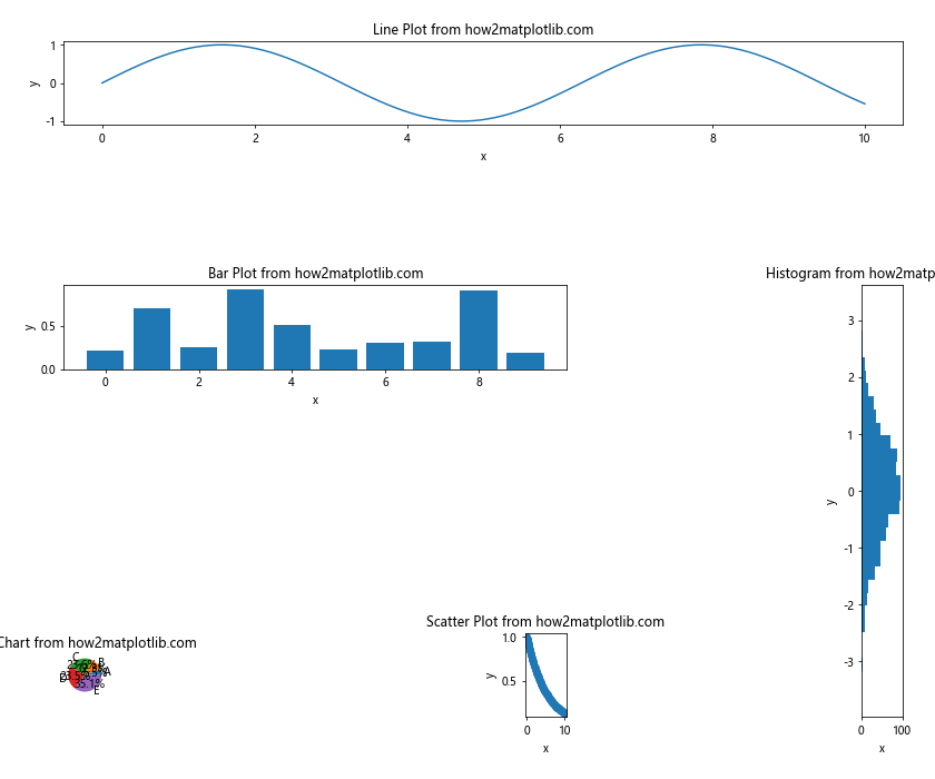
In this example, we create a complex layout with different types of plots, including a line plot, bar plot, histogram, pie chart, and scatter plot. By using Matplotlib.figure.Figure.set_constrained_layout_pads(), we can adjust the padding and spacing to ensure that all plots are properly arranged and visible, despite their different sizes and shapes.
Fine-tuning Matplotlib.figure.Figure.set_constrained_layout_pads() for Publication-Quality Figures
When preparing figures for publication, you may need to adjust the padding and spacing to meet specific requirements. Let’s look at an example of how to use Matplotlib.figure.Figure.set_constrained_layout_pads() to create publication-quality figures:
import matplotlib.pyplot as plt
import numpy as np

# Set the figure style for publication
plt.style.use('seaborn-whitegrid')

# Create a figure with constrained layout
fig, axs = plt.subplots(2, 2, constrained_layout=True, figsize=(10, 8))

# Generate some sample data
x = np.linspace(0, 10, 100)
y1 = np.sin(x)
y2 = np.cos(x)
y3 = np.tan(x)
y4 = np.exp(-x/5)

# Plot the data
axs[0, 0].plot(x, y1, label='sin(x)')
axs[0, 1].plot(x, y2, label='cos(x)')
axs[1, 0].plot(x, y3, label='tan(x)')
axs[1, 1].plot(x, y4, label='exp(-x/5)')

# Add labels and titles
for ax in axs.flat:
    ax.set_xlabel('x', fontsize=12)
    ax.set_ylabel('y', fontsize=12)
    ax.legend(fontsize=10)
    ax.set_title('Plot from how2matplotlib.com', fontsize=14)
    ax.tick_params(axis='both', which='major', labelsize=10)

# Add a main title to the figure
fig.suptitle('Publication-Quality Plots', fontsize=16)

# Set constrained layout pads for optimal spacing
fig.set_constrained_layout_pads(w_pad=0.2, h_pad=0.3, wspace=0.3, hspace=0.3)

# Adjust the overall layout
plt.tight_layout(rect=[0, 0.03, 1, 0.95])

plt.show()
In this example, we create a 2×2 grid of subplots with a publication-quality style. We use Matplotlib.figure.Figure.set_constrained_layout_pads() to fine-tune the padding and spacing, ensuring that all elements are properly positioned and easily readable. We also add a main title to the figure and adjust the font sizes for better visibility.
Conclusion
Matplotlib.figure.Figure.set_constrained_layout_pads() is a powerful tool for optimizing the layout of your plots in Python. By adjusting the padding and spacing parameters, you can create visually appealing and well-organized figures that effectively communicate your data. Throughout this article, we’ve explored various examples and use cases for Matplotlib.figure.Figure.set_constrained_layout_pads(), demonstrating its versatility in handling different plot types, layouts, and requirements.
Some key takeaways from our exploration of Matplotlib.figure.Figure.set_constrained_layout_pads() include:
- The method allows you to fine-tune the padding around subplots and the figure edges.
- It’s particularly useful when working with complex layouts, multiple subplots, or plots with additional elements like colorbars and legends.
- You can adapt the padding parameters for different figure sizes and aspect ratios to ensure optimal layout across various display contexts.
- Matplotlib.figure.Figure.set_constrained_layout_pads() can help you create publication-quality figures by allowing precise control over spacing and alignment.
By mastering the use of Matplotlib.figure.Figure.set_constrained_layout_pads(), you’ll be able to create more professional and visually appealing plots that effectively showcase your data and analysis. Remember to experiment with different padding values to find the optimal layout for your specific plots and requirements.