How to Use Matplotlib.artist.Artist.set_clip_box() in Python
Matplotlib.artist.Artist.set_clip_box() in Python is a powerful method that allows you to control the visibility of artists in your plots. This function is an essential tool for creating more sophisticated and visually appealing visualizations. In this comprehensive guide, we’ll explore the ins and outs of Matplotlib.artist.Artist.set_clip_box(), providing you with detailed explanations and practical examples to help you master this technique.
Understanding Matplotlib.artist.Artist.set_clip_box()
Matplotlib.artist.Artist.set_clip_box() is a method that belongs to the Artist class in Matplotlib. It is used to set the clipping box for an artist, which determines the region where the artist will be visible. Any part of the artist that falls outside this clipping box will be hidden from view.
The syntax for using Matplotlib.artist.Artist.set_clip_box() is as follows:
artist.set_clip_box(clipbox)
Where artist is the Matplotlib artist object you want to clip, and clipbox is a matplotlib.transforms.Bbox object that defines the clipping region.
Let’s dive deeper into how to use Matplotlib.artist.Artist.set_clip_box() effectively in your Python projects.
Creating a Basic Plot with Matplotlib.artist.Artist.set_clip_box()
To get started with Matplotlib.artist.Artist.set_clip_box(), let’s create a simple plot and apply clipping to it. Here’s an example:
import matplotlib.pyplot as plt
import numpy as np
from matplotlib.transforms import Bbox

# Create data for the plot
x = np.linspace(0, 10, 100)
y = np.sin(x)

# Create the plot
fig, ax = plt.subplots()
line, = ax.plot(x, y, label='Sine wave')

# Define the clipping box
clip_box = Bbox([[2, -0.5], [8, 0.5]])

# Apply the clipping box to the line
line.set_clip_box(clip_box)

# Set labels and title
ax.set_xlabel('X-axis')
ax.set_ylabel('Y-axis')
ax.set_title('Clipped Sine Wave - how2matplotlib.com')

# Add legend
ax.legend()

# Show the plot
plt.show()
Output:
In this example, we create a simple sine wave plot and then use Matplotlib.artist.Artist.set_clip_box() to clip the line to a specific region. The clipping box is defined using a Bbox object, which specifies the lower-left and upper-right corners of the box.
Understanding the Bbox Object
The Bbox (Bounding Box) object is crucial when working with Matplotlib.artist.Artist.set_clip_box(). It defines a rectangular region in the plot coordinates. Let’s explore how to create and manipulate Bbox objects:
import matplotlib.pyplot as plt
from matplotlib.transforms import Bbox

# Create a figure and axis
fig, ax = plt.subplots()

# Create a Bbox object
bbox = Bbox([[1, 1], [3, 3]])

# Draw the Bbox on the plot
rect = plt.Rectangle((bbox.xmin, bbox.ymin), bbox.width, bbox.height,
                     fill=False, edgecolor='r', linewidth=2)
ax.add_patch(rect)

# Set labels and title
ax.set_xlabel('X-axis')
ax.set_ylabel('Y-axis')
ax.set_title('Bbox Visualization - how2matplotlib.com')

# Set axis limits
ax.set_xlim(0, 4)
ax.set_ylim(0, 4)

# Show the plot
plt.show()
Output:
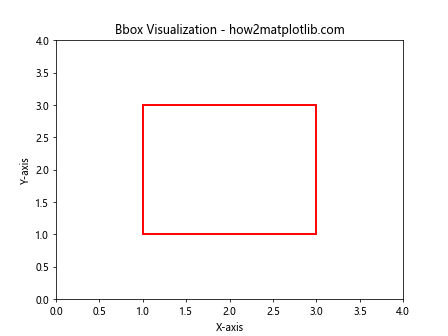
This example demonstrates how to create a Bbox object and visualize it on a plot. Understanding how to work with Bbox objects is essential for effectively using Matplotlib.artist.Artist.set_clip_box().
Applying Matplotlib.artist.Artist.set_clip_box() to Different Plot Types
Matplotlib.artist.Artist.set_clip_box() can be applied to various types of plots. Let’s explore how to use it with different plot types:
Line Plots
import matplotlib.pyplot as plt
import numpy as np
from matplotlib.transforms import Bbox

# Create data for the plot
x = np.linspace(0, 10, 100)
y1 = np.sin(x)
y2 = np.cos(x)

# Create the plot
fig, ax = plt.subplots()
line1, = ax.plot(x, y1, label='Sine')
line2, = ax.plot(x, y2, label='Cosine')

# Define the clipping box
clip_box = Bbox([[2, -0.5], [8, 0.5]])

# Apply the clipping box to both lines
line1.set_clip_box(clip_box)
line2.set_clip_box(clip_box)

# Set labels and title
ax.set_xlabel('X-axis')
ax.set_ylabel('Y-axis')
ax.set_title('Clipped Sine and Cosine Waves - how2matplotlib.com')

# Add legend
ax.legend()

# Show the plot
plt.show()
Output:
In this example, we apply Matplotlib.artist.Artist.set_clip_box() to two line plots, clipping both the sine and cosine waves to the same region.
Scatter Plots
import matplotlib.pyplot as plt
import numpy as np
from matplotlib.transforms import Bbox

# Create data for the scatter plot
np.random.seed(42)
x = np.random.rand(100)
y = np.random.rand(100)

# Create the scatter plot
fig, ax = plt.subplots()
scatter = ax.scatter(x, y, c=y, cmap='viridis')

# Define the clipping box
clip_box = Bbox([[0.25, 0.25], [0.75, 0.75]])

# Apply the clipping box to the scatter plot
scatter.set_clip_box(clip_box)

# Set labels and title
ax.set_xlabel('X-axis')
ax.set_ylabel('Y-axis')
ax.set_title('Clipped Scatter Plot - how2matplotlib.com')

# Add colorbar
plt.colorbar(scatter)

# Show the plot
plt.show()
Output:
This example demonstrates how to apply Matplotlib.artist.Artist.set_clip_box() to a scatter plot, limiting the visible points to a specific region.
Bar Plots
import matplotlib.pyplot as plt
import numpy as np
from matplotlib.transforms import Bbox

# Create data for the bar plot
categories = ['A', 'B', 'C', 'D', 'E']
values = [3, 7, 2, 5, 8]

# Create the bar plot
fig, ax = plt.subplots()
bars = ax.bar(categories, values)

# Define the clipping box
clip_box = Bbox([[1, 0], [4, 6]])

# Apply the clipping box to each bar
for bar in bars:
    bar.set_clip_box(clip_box)

# Set labels and title
ax.set_xlabel('Categories')
ax.set_ylabel('Values')
ax.set_title('Clipped Bar Plot - how2matplotlib.com')

# Show the plot
plt.show()
Output:
In this example, we apply Matplotlib.artist.Artist.set_clip_box() to a bar plot, clipping the bars to a specific region.
Advanced Techniques with Matplotlib.artist.Artist.set_clip_box()
Now that we’ve covered the basics, let’s explore some advanced techniques for using Matplotlib.artist.Artist.set_clip_box():
Dynamic Clipping
You can create dynamic clipping effects by updating the clip box in real-time. Here’s an example that demonstrates this:
import matplotlib.pyplot as plt
import numpy as np
from matplotlib.transforms import Bbox
from matplotlib.animation import FuncAnimation

# Create data for the plot
x = np.linspace(0, 10, 100)
y = np.sin(x)

# Create the plot
fig, ax = plt.subplots()
line, = ax.plot(x, y)

# Initialize the clipping box
clip_box = Bbox([[0, -1], [10, 1]])
line.set_clip_box(clip_box)

# Animation update function
def update(frame):
    clip_box.x0 = frame / 10
    clip_box.x1 = 10 - frame / 10
    line.set_clip_box(clip_box)
    return line,

# Create the animation
anim = FuncAnimation(fig, update, frames=100, interval=50, blit=True)

# Set labels and title
ax.set_xlabel('X-axis')
ax.set_ylabel('Y-axis')
ax.set_title('Dynamic Clipping - how2matplotlib.com')

# Show the plot
plt.show()
Output:
This example creates an animation where the clipping box for a sine wave changes dynamically, creating a moving window effect.
Clipping with Custom Shapes
While Matplotlib.artist.Artist.set_clip_box() typically uses rectangular clipping regions, you can achieve more complex clipping shapes by combining it with other Matplotlib features. Here’s an example that demonstrates circular clipping:
import matplotlib.pyplot as plt
import numpy as np
from matplotlib.patches import Circle

# Create data for the plot
x = np.linspace(-5, 5, 100)
y = np.linspace(-5, 5, 100)
X, Y = np.meshgrid(x, y)
Z = np.sin(np.sqrt(X**2 + Y**2))

# Create the plot
fig, ax = plt.subplots()
im = ax.imshow(Z, extent=[-5, 5, -5, 5], origin='lower', cmap='viridis')

# Create a circular clipping patch
circle = Circle((0, 0), radius=3, transform=ax.transData)
im.set_clip_path(circle)

# Set labels and title
ax.set_xlabel('X-axis')
ax.set_ylabel('Y-axis')
ax.set_title('Circular Clipping - how2matplotlib.com')

# Add colorbar
plt.colorbar(im)

# Show the plot
plt.show()
Output:
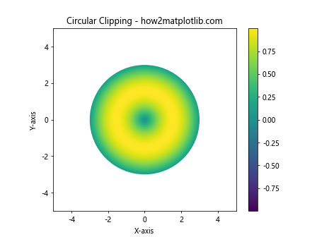
In this example, we use a circular patch as a clipping path to create a circular clipping effect on an image plot.
Combining Matplotlib.artist.Artist.set_clip_box() with Other Matplotlib Features
Matplotlib.artist.Artist.set_clip_box() can be combined with other Matplotlib features to create more complex visualizations. Let’s explore some examples:
Clipping with Subplots
import matplotlib.pyplot as plt
import numpy as np
from matplotlib.transforms import Bbox

# Create data for the plots
x = np.linspace(0, 10, 100)
y1 = np.sin(x)
y2 = np.cos(x)

# Create a figure with two subplots
fig, (ax1, ax2) = plt.subplots(1, 2, figsize=(12, 5))

# Plot in the first subplot
line1, = ax1.plot(x, y1)
clip_box1 = Bbox([[2, -0.5], [8, 0.5]])
line1.set_clip_box(clip_box1)
ax1.set_title('Clipped Sine Wave - how2matplotlib.com')

# Plot in the second subplot
line2, = ax2.plot(x, y2)
clip_box2 = Bbox([[4, -0.5], [6, 0.5]])
line2.set_clip_box(clip_box2)
ax2.set_title('Clipped Cosine Wave - how2matplotlib.com')

# Adjust layout and show the plot
plt.tight_layout()
plt.show()
Output:
This example demonstrates how to use Matplotlib.artist.Artist.set_clip_box() with subplots, applying different clipping regions to each subplot.
Clipping with Custom Colormaps
import matplotlib.pyplot as plt
import numpy as np
from matplotlib.transforms import Bbox
from matplotlib.colors import LinearSegmentedColormap

# Create data for the plot
x = np.linspace(0, 10, 100)
y = np.linspace(0, 10, 100)
X, Y = np.meshgrid(x, y)
Z = np.sin(X) * np.cos(Y)

# Create a custom colormap
colors = ['blue', 'white', 'red']
n_bins = 100
cmap = LinearSegmentedColormap.from_list('custom_cmap', colors, N=n_bins)

# Create the plot
fig, ax = plt.subplots()
im = ax.imshow(Z, extent=[0, 10, 0, 10], origin='lower', cmap=cmap)

# Define the clipping box
clip_box = Bbox([[2, 2], [8, 8]])

# Apply the clipping box to the image
im.set_clip_box(clip_box)

# Set labels and title
ax.set_xlabel('X-axis')
ax.set_ylabel('Y-axis')
ax.set_title('Clipped Image with Custom Colormap - how2matplotlib.com')

# Add colorbar
plt.colorbar(im)

# Show the plot
plt.show()
Output:
This example combines Matplotlib.artist.Artist.set_clip_box() with a custom colormap to create a visually striking clipped image plot.
Best Practices for Using Matplotlib.artist.Artist.set_clip_box()
When working with Matplotlib.artist.Artist.set_clip_box(), keep these best practices in mind:
- Always define the clipping box in data coordinates unless you have a specific reason to use other coordinate systems.
- Be mindful of the plot limits when setting the clipping box to ensure that the clipped region is visible.
- When clipping multiple artists, consider using the same clipping box for consistency.
- Use Matplotlib.artist.Artist.set_clip_box() in combination with other Matplotlib features to create more sophisticated visualizations.
- Remember that clipping affects only the visibility of the artist, not its underlying data or properties.
Troubleshooting Common Issues with Matplotlib.artist.Artist.set_clip_box()
When using Matplotlib.artist.Artist.set_clip_box(), you might encounter some common issues. Here are some troubleshooting tips:
Issue: Clipping Not Visible
If the clipping effect is not visible, check the following:
- Ensure that the clipping box is within the visible range of your plot.
- Verify that the artist you’re trying to clip is actually visible in the plot.
Here’s an example that demonstrates how to debug this issue:
import matplotlib.pyplot as plt
import numpy as np
from matplotlib.transforms import Bbox

# Create data for the plot
x = np.linspace(0, 10, 100)
y = np.sin(x)

# Create the plot
fig, ax = plt.subplots()
line, = ax.plot(x, y)

# Define the clipping box
clip_box = Bbox([[2, -0.5], [8, 0.5]])

# Apply the clipping box to the line
line.set_clip_box(clip_box)

# Set labels and title
ax.set_xlabel('X-axis')
ax.set_ylabel('Y-axis')
ax.set_title('Debugging Clipping - how2matplotlib.com')

# Add the clipping box visualization
rect = plt.Rectangle((clip_box.xmin, clip_box.ymin), clip_box.width, clip_box.height,
                     fill=False, edgecolor='r', linewidth=2)
ax.add_patch(rect)

# Show the plot
plt.show()
Output:
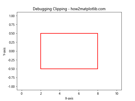
This example adds a visual representation of the clipping box to help you debug any issues with visibility.
Issue: Unexpected Clipping Behavior
If you’re experiencing unexpected clipping behavior, it might be due to coordinate system mismatches. Ensure that you’re using the correct coordinate system for your clipping box. Here’s an example that demonstrates how to use different coordinate systems:
import matplotlib.pyplot as plt
import numpy as np
from matplotlib.transforms import Bbox

# Create data for the plot
x = np.linspace(0, 10, 100)
y = np.sin(x)

# Create the plot
fig, ax = plt.subplots()
line, = ax.plot(x, y)

# Define clipping boxes in different coordinate systems
data_clip_box = Bbox([[2, -0.5], [8, 0.5]])
axes_clip_box = Bbox([[0.2, 0.2], [0.8, 0.8]])

# Apply the clipping boxes
line.set_clip_box(data_clip_box)  # Data coordinates
ax.set_clip_box(axes_clip_box)    # Axes coordinates

# Set labels and title
ax.set_xlabel('X-axis')
ax.set_ylabel('Y-axis')
ax.set_title('Clipping in Different Coordinate Systems - how2matplotlib.com')

# Visualize the clipping boxes
data_rect = plt.Rectangle((data_clip_box.xmin, data_clip_box.ymin), data_clip_box.width, data_clip_box.height,
                          fill=False, edgecolor='r', linewidth=2, label='Data Clip Box')
axes_rect = plt.Rectangle((axes_clip_box.xmin, axes_clip_box.ymin), axes_clip_box.width, axes_clip_box.height,
                          fill=False, edgecolor='g', linewidth=2, label='Axes Clip Box', transform=ax.transAxes)
ax.add_patch(data_rect)
ax.add_patch(axes_rect)

# Add legend
ax.legend()

# Show the plot
plt.show()
Output:
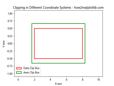
This example demonstrates how to use clipping boxes in both data and axes coordinates, helping you understand and debug coordinate system-related issues.
Advanced Applications of Matplotlib.artist.Artist.set_clip_box()
Now that we’ve covered the basics and troubleshooting, let’s explore some advanced applications of Matplotlib.artist.Artist.set_clip_box():
Creating a Magnifying Glass Effect
You can use Matplotlib.artist.Artist.set_clip_box() to create a magnifying glass effect on your plots. Here’s an example:
import matplotlib.pyplot as plt
import numpy as np
from matplotlib.transforms import Bbox
from matplotlib.patches import Circle

# Create data for the plot
x = np.linspace(0, 10, 1000)
y = np.sin(x) + np.random.normal(0, 0.1, 1000)

# Create the plot
fig, ax = plt.subplots(figsize=(10, 6))
line, = ax.plot(x, y, alpha=0.5)

# Create a magnified version of the plot
ax_inset = ax.inset_axes([0.5, 0.5, 0.47, 0.47])
line_mag, = ax_inset.plot(x, y)

# Set the limits for the magnified area
xlim = (4, 6)
ylim = (-0.5, 1.5)
ax_inset.set_xlim(xlim)
ax_inset.set_ylim(ylim)

# Create a circular clipping path for the magnified plot
circle = Circle((0.5, 0.5), 0.5, transform=ax_inset.transAxes, fill=False, edgecolor='r', linewidth=2)
line_mag.set_clip_path(circle)

# Add connecting lines
ax.indicate_inset_zoom(ax_inset, edgecolor="black")

# Set labels and title
ax.set_xlabel('X-axis')
ax.set_ylabel('Y-axis')
ax.set_title('Magnifying Glass Effect - how2matplotlib.com')

# Show the plot
plt.show()
Output:
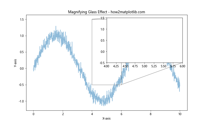
This example creates a magnifying glass effect by using an inset axes and applying a circular clipping path to the magnified plot.
Creating a Reveal Animation
You can use Matplotlib.artist.Artist.set_clip_box() to create a reveal animation that gradually uncovers a plot. Here’s an example:
import matplotlib.pyplot as plt
import numpy as np
from matplotlib.transforms import Bbox
from matplotlib.animation import FuncAnimation

# Create data for the plot
x = np.linspace(0, 10, 100)
y = np.sin(x)

# Create the plot
fig, ax = plt.subplots()
line, = ax.plot(x, y)

# Initialize the clipping box
clip_box = Bbox([[0, -1], [0, 1]])
line.set_clip_box(clip_box)

# Animation update function
def update(frame):
    clip_box.x1 = frame / 10
    line.set_clip_box(clip_box)
    return line,

# Create the animation
anim = FuncAnimation(fig, update, frames=100, interval=50, blit=True)

# Set labels and title
ax.set_xlabel('X-axis')
ax.set_ylabel('Y-axis')
ax.set_title('Reveal Animation - how2matplotlib.com')

# Show the plot
plt.show()
Output:
This example creates an animation that gradually reveals a sine wave plot from left to right using Matplotlib.artist.Artist.set_clip_box().
Comparing Matplotlib.artist.Artist.set_clip_box() with Other Clipping Methods
While Matplotlib.artist.Artist.set_clip_box() is a powerful tool for clipping artists, Matplotlib offers other clipping methods as well. Let’s compare it with some alternatives:
set_clip_box() vs. set_clip_path()
import matplotlib.pyplot as plt
import numpy as np
from matplotlib.transforms import Bbox
from matplotlib.patches import Circle

# Create data for the plot
x = np.linspace(0, 10, 100)
y = np.sin(x)

# Create the plot
fig, (ax1, ax2) = plt.subplots(1, 2, figsize=(12, 5))

# Plot with set_clip_box()
line1, = ax1.plot(x, y)
clip_box = Bbox([[2, -0.5], [8, 0.5]])
line1.set_clip_box(clip_box)
ax1.set_title('set_clip_box() - how2matplotlib.com')

# Plot with set_clip_path()
line2, = ax2.plot(x, y)
circle = Circle((5, 0), radius=2, transform=ax2.transData)
line2.set_clip_path(circle)
ax2.set_title('set_clip_path() - how2matplotlib.com')

# Set labels
for ax in (ax1, ax2):
    ax.set_xlabel('X-axis')
    ax.set_ylabel('Y-axis')

# Adjust layout and show the plot
plt.tight_layout()
plt.show()
Output:
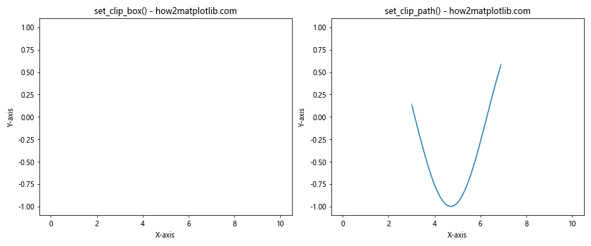
This example compares Matplotlib.artist.Artist.set_clip_box() with set_clip_path(), demonstrating how set_clip_path() allows for more complex clipping shapes.
set_clip_box() vs. set_xlim() and set_ylim()
import matplotlib.pyplot as plt
import numpy as np
from matplotlib.transforms import Bbox

# Create data for the plot
x = np.linspace(0, 10, 100)
y = np.sin(x)

# Create the plot
fig, (ax1, ax2) = plt.subplots(1, 2, figsize=(12, 5))

# Plot with set_clip_box()
line1, = ax1.plot(x, y)
clip_box = Bbox([[2, -0.5], [8, 0.5]])
line1.set_clip_box(clip_box)
ax1.set_title('set_clip_box() - how2matplotlib.com')

# Plot with set_xlim() and set_ylim()
line2, = ax2.plot(x, y)
ax2.set_xlim(2, 8)
ax2.set_ylim(-0.5, 0.5)
ax2.set_title('set_xlim() and set_ylim() - how2matplotlib.com')

# Set labels
for ax in (ax1, ax2):
    ax.set_xlabel('X-axis')
    ax.set_ylabel('Y-axis')

# Adjust layout and show the plot
plt.tight_layout()
plt.show()
Output:
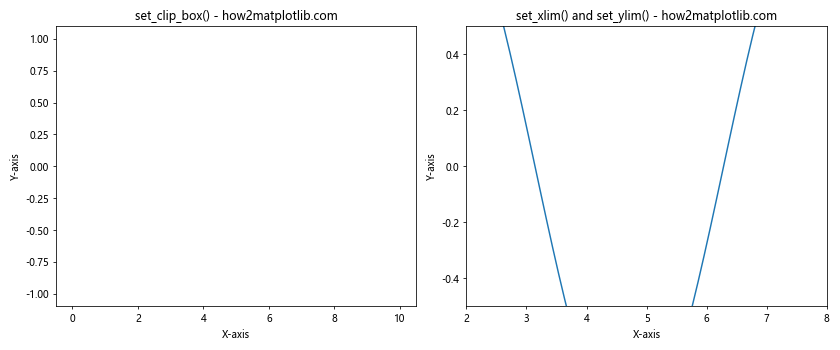
This example compares Matplotlib.artist.Artist.set_clip_box() with using set_xlim() and set_ylim() to limit the visible area of a plot.
Conclusion
Matplotlib.artist.Artist.set_clip_box() is a versatile and powerful tool for controlling the visibility of artists in Matplotlib plots. Throughout this comprehensive guide, we’ve explored its basic usage, advanced techniques, troubleshooting tips, and comparisons with other clipping methods.
By mastering Matplotlib.artist.Artist.set_clip_box(), you can create more sophisticated and visually appealing plots, implement dynamic clipping effects, and combine it with other Matplotlib features to achieve complex visualizations.
Remember to consider the coordinate systems when defining clipping boxes, and don’t hesitate to experiment with different shapes and animations to create unique and engaging plots.