Matplotlib 3D Contours

Matplotlib 3D Contours

Matplotlib is a comprehensive library for creating static, animated, and interactive visualizations in Python. It offers an array of tools for data visualization, including 3D plotting capabilities which can be particularly useful for visualizing complex datasets. One of the 3D plotting techniques available in Matplotlib is 3D contour plotting. This technique is valuable for understanding the relationships among three-dimensional data points. In this article, we will explore how to create 3D contour plots using Matplotlib, providing detailed examples to illustrate the process.

Introduction to 3D Contour Plots

A 3D contour plot is a method to plot contours of a three-dimensional surface on a three-dimensional plot. These contours represent slices or cross-sections of the surface at different heights. This type of visualization can help in understanding the topography of a surface, identifying patterns, and analyzing the distribution of data points in three-dimensional space.

To create 3D contour plots in Matplotlib, we primarily use the contour and contourf functions from the mplot3d toolkit. Before diving into the examples, ensure you have Matplotlib installed in your environment. If not, you can install it using pip:

pip install matplotlib

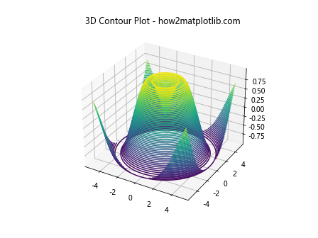
Basic 3D Contour Plot

Let’s start with a basic example of a 3D contour plot. This example will demonstrate how to create a simple 3D contour plot using synthetic data.

import matplotlib.pyplot as plt
from mpl_toolkits.mplot3d import Axes3D
import numpy as np

x = np.linspace(-5, 5, 100)
y = np.linspace(-5, 5, 100)
x, y = np.meshgrid(x, y)
z = np.sin(np.sqrt(x**2 + y**2))

fig = plt.figure()
ax = fig.add_subplot(111, projection='3d')
ax.contour3D(x, y, z, 50)
ax.set_title('3D Contour Plot - how2matplotlib.com')
plt.show()

Output:

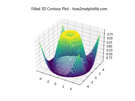
Filled 3D Contour Plot

Filled contour plots (contourf) can provide a better visual representation by filling the space between the contours with colors.

import matplotlib.pyplot as plt
from mpl_toolkits.mplot3d import Axes3D
import numpy as np

x = np.linspace(-5, 5, 100)
y = np.linspace(-5, 5, 100)
x, y = np.meshgrid(x, y)
z = np.sin(np.sqrt(x**2 + y**2))

fig = plt.figure()
ax = fig.add_subplot(111, projection='3d')
ax.contourf(x, y, z, 50)
ax.set_title('Filled 3D Contour Plot - how2matplotlib.com')
plt.show()

Output:

Customizing Contour Plots

Customization is key to making plots more informative and visually appealing. Here’s how you can customize the appearance of 3D contour plots.

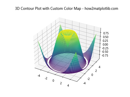
Changing the Color Map

import matplotlib.pyplot as plt
from mpl_toolkits.mplot3d import Axes3D
import numpy as np

x = np.linspace(-5, 5, 100)
y = np.linspace(-5, 5, 100)
x, y = np.meshgrid(x, y)
z = np.sin(np.sqrt(x**2 + y**2))

fig = plt.figure()
ax = fig.add_subplot(111, projection='3d')
ax.contour3D(x, y, z, 50, cmap='viridis')
ax.set_title('3D Contour Plot with Custom Color Map - how2matplotlib.com')
plt.show()

Output:

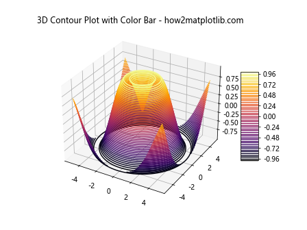
Adding Color Bar

import matplotlib.pyplot as plt
from mpl_toolkits.mplot3d import Axes3D
import numpy as np

x = np.linspace(-5, 5, 100)
y = np.linspace(-5, 5, 100)
x, y = np.meshgrid(x, y)
z = np.sin(np.sqrt(x**2 + y**2))

fig = plt.figure()
ax = fig.add_subplot(111, projection='3d')
contour = ax.contour3D(x, y, z, 50, cmap='inferno')
fig.colorbar(contour, ax=ax, shrink=0.5, aspect=5)
ax.set_title('3D Contour Plot with Color Bar - how2matplotlib.com')
plt.show()

Output:

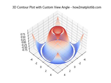
Adjusting the View Angle

import matplotlib.pyplot as plt
from mpl_toolkits.mplot3d import Axes3D
import numpy as np

x = np.linspace(-5, 5, 100)
y = np.linspace(-5, 5, 100)
x, y = np.meshgrid(x, y)
z = np.sin(np.sqrt(x**2 + y**2))

fig = plt.figure()
ax = fig.add_subplot(111, projection='3d')
ax.contour3D(x, y, z, 50, cmap='coolwarm')
ax.view_init(elev=45, azim=45)
ax.set_title('3D Contour Plot with Custom View Angle - how2matplotlib.com')
plt.show()

Output:

Advanced Examples

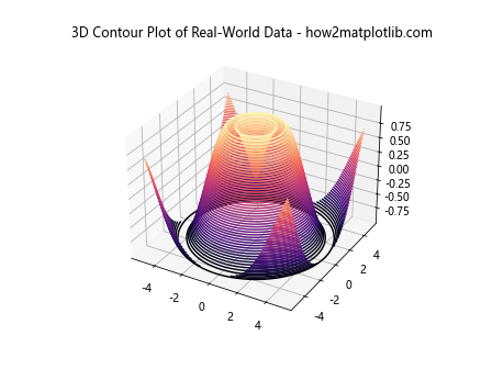
Plotting Real-World Data

Real-world data often comes in irregular shapes and sizes. Here’s how you might visualize such data using 3D contour plots.

import matplotlib.pyplot as plt
from mpl_toolkits.mplot3d import Axes3D
import numpy as np

x = np.linspace(-5, 5, 100)
y = np.linspace(-5, 5, 100)
x, y = np.meshgrid(x, y)
z = np.sin(np.sqrt(x**2 + y**2))

# This example assumes you have real-world data loaded into x, y, z variables
fig = plt.figure()
ax = fig.add_subplot(111, projection='3d')
ax.contour3D(x, y, z, 50, cmap='magma')
ax.set_title('3D Contour Plot of Real-World Data - how2matplotlib.com')
plt.show()

Output:

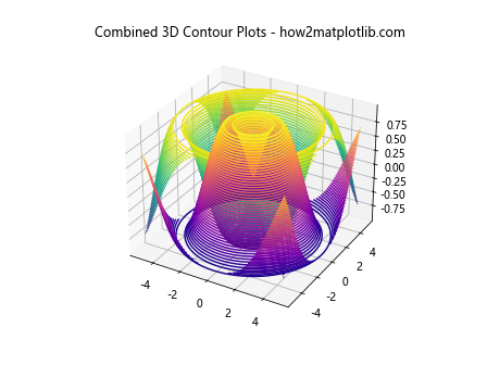
Combining Multiple Contour Plots

Sometimes, you might want to combine multiple contour plots for comparison or to highlight different aspects of the data.

import matplotlib.pyplot as plt
from mpl_toolkits.mplot3d import Axes3D
import numpy as np

x = np.linspace(-5, 5, 100)
y = np.linspace(-5, 5, 100)
x, y = np.meshgrid(x, y)
z = np.sin(np.sqrt(x**2 + y**2))

fig = plt.figure()
ax = fig.add_subplot(111, projection='3d')
ax.contour3D(x, y, z, 50, cmap='plasma')
ax.contour3D(x, y, -z, 50, cmap='viridis')
ax.set_title('Combined 3D Contour Plots - how2matplotlib.com')
plt.show()

Output:

Interactive 3D Contour Plots

Interactive plots allow users to explore the data by rotating, zooming, and panning the plot. Matplotlib’s notebook backend supports interactive plots in Jupyter notebooks.

%matplotlib notebook
import matplotlib.pyplot as plt
from mpl_toolkits.mplot3d import Axes3D
import numpy as np

# Your plotting code here

Conclusion

3D contour plots are a powerful tool for visualizing complex datasets in three dimensions. By leveraging the capabilities of Matplotlib, you can create detailed and informative visualizations that help in understanding the underlying patterns and relationships within your data. The examples provided in this article serve as a starting point, but the true potential of Matplotlib’s 3D plotting capabilities is limited only by your imagination and the specific requirements of your data analysis tasks.