Using ax.annotate in Matplotlib

Using ax.annotate in Matplotlib

Matplotlib is a powerful library in Python for creating visualizations and plots. One important feature of Matplotlib is the ax.annotate() function, which can be used to add annotations to plots. Annotations can help explain key points or features of the data being plotted, making the visualization more informative and easier to understand.

In this article, we will explore how to use the ax.annotate() function in Matplotlib to add annotations to various types of plots. We will cover different ways to customize the annotations and make them stand out in the plot.

Basic Annotations

The ax.annotate() function in Matplotlib can be used to add text annotations at specified positions in a plot. The basic syntax of ax.annotate() is:

import matplotlib.pyplot as plt

fig, ax = plt.subplots()

ax.plot([1, 2, 3, 4], [1, 4, 9, 16])
ax.annotate('Example Annotation', (2, 4))

plt.show()

Output:

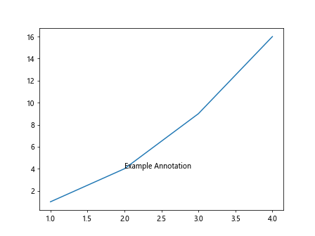
In this example, we create a simple line plot and add an annotation with the text ‘Example Annotation’ at the point (2, 4) in the plot.

Customizing Annotations

Text Properties

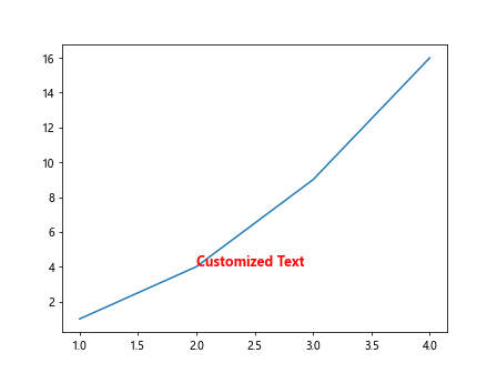
You can customize the appearance of the text in the annotation by specifying the fontsize, color, fontstyle, and fontweight properties. Here’s an example:

import matplotlib.pyplot as plt

fig, ax = plt.subplots()

ax.plot([1, 2, 3, 4], [1, 4, 9, 16])
ax.annotate('Customized Text', (2, 4),
            fontsize=12, color='red', fontstyle='italic', fontweight='bold')

plt.show()

Output:

Arrow Properties

You can also add an arrow to point to the annotated position by setting the arrowprops parameter. Here’s an example:

import matplotlib.pyplot as plt

fig, ax = plt.subplots()

ax.plot([1, 2, 3, 4], [1, 4, 9, 16])
ax.annotate('Annotation with Arrow', (2, 4),
            arrowprops=dict(facecolor='blue', arrowstyle='->'))

plt.show()

Output:

Background Color

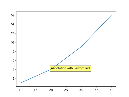
You can add a background color to the annotation text by setting the bbox parameter. Here’s an example:

import matplotlib.pyplot as plt

fig, ax = plt.subplots()

ax.plot([1, 2, 3, 4], [1, 4, 9, 16])
ax.annotate('Annotation with Background', (2, 4),
            bbox=dict(facecolor='yellow', alpha=0.5))

plt.show()

Output:

Annotations on Different Types of Plots

Line Plot

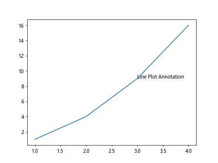
You can add annotations to line plots by specifying the x and y coordinates for the annotation position. Here’s an example:

import matplotlib.pyplot as plt

fig, ax = plt.subplots()

x = [1, 2, 3, 4]
y = [1, 4, 9, 16]

ax.plot(x, y)
ax.annotate('Line Plot Annotation', (x[2], y[2]))

plt.show()

Output:

Scatter Plot

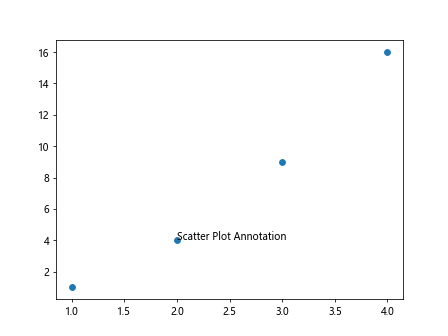
You can add annotations to scatter plots by specifying the x and y coordinates for the annotation position. Here’s an example:

import matplotlib.pyplot as plt

fig, ax = plt.subplots()

x = [1, 2, 3, 4]
y = [1, 4, 9, 16]

ax.scatter(x, y)
ax.annotate('Scatter Plot Annotation', (x[1], y[1]))

plt.show()

Output:

Bar Plot

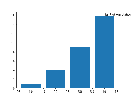
You can add annotations to bar plots by specifying the x and y coordinates for the annotation position. Here’s an example:

import matplotlib.pyplot as plt

fig, ax = plt.subplots()

x = [1, 2, 3, 4]
y = [1, 4, 9, 16]

ax.bar(x, y)
ax.annotate('Bar Plot Annotation', (x[3], y[3]))

plt.show()

Output:

Pie Chart

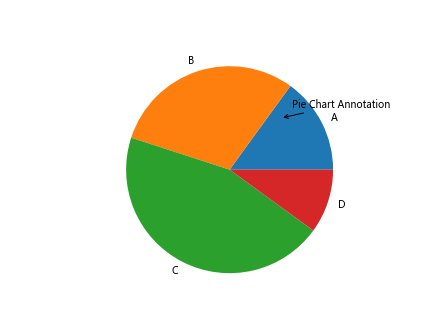
You can add annotations to pie charts by specifying the angle and radius for the annotation position. Here’s an example:

import matplotlib.pyplot as plt

fig, ax = plt.subplots()

sizes = [15, 30, 45, 10]
labels = ['A', 'B', 'C', 'D']

ax.pie(sizes, labels=labels)
ax.annotate('Pie Chart Annotation', xy=(0.5, 0.5), xytext=(0.6, 0.6),
            arrowprops=dict(facecolor='black', arrowstyle='->'))

plt.show()

Output:

Annotation with LaTeX Math

You can use LaTeX math expressions in annotations by setting the usetex parameter to True. Here’s an example:

import matplotlib.pyplot as plt

fig, ax = plt.subplots()

ax.plot([1, 2, 3, 4], [1, 4, 9, 16])
ax.annotate(r'\sum_{i=1}^{N} x_i', (2, 4), fontsize=12, usetex=True)

plt.show()

ax.annotate Conclusion

In this article, we have explored how to use the ax.annotate() function in Matplotlib to add annotations to plots. We have covered various customization options such as text properties, arrow properties, background color, and annotations on different types of plots including line plots, scatter plots, bar plots, and pie charts. We have also seen how to use LaTeX math expressions in annotations. Annotations can enhance the clarity and visual appeal of your plots, making them more informative and easier to interpret. Experiment with different customization options and types of plots to create visually appealing and informative visualizations with annotations in Matplotlib.