Ax Annotate in Matplotlib

Ax Annotate in Matplotlib

Introduction

In Matplotlib, the annotate method in the Axes class can be used to add annotations to plots. Annotations can be used to highlight important points or add additional information to the plot. This article will provide a detailed overview of how to use the annotate method in Matplotlib.

Adding Annotations

To add annotations to a plot in Matplotlib, we can use the annotate method in the Axes class. The general syntax for the annotate method is as follows:

ax.annotate(text, xy, xytext, arrowprops)

• text: The text of the annotation.
• xy: The point being annotated.
• xytext: The location of the text.
• arrowprops: Properties for the arrow that connects the annotation to the point.

Here is an example of adding a simple annotation to a plot:

import matplotlib.pyplot as plt

fig, ax = plt.subplots()
ax.plot([1, 2, 3], [4, 5, 6])
ax.annotate('Important Point', xy=(2, 5), xytext=(2.5, 5.5),
            arrowprops=dict(facecolor='red', shrink=0.05))
plt.show()

Output:

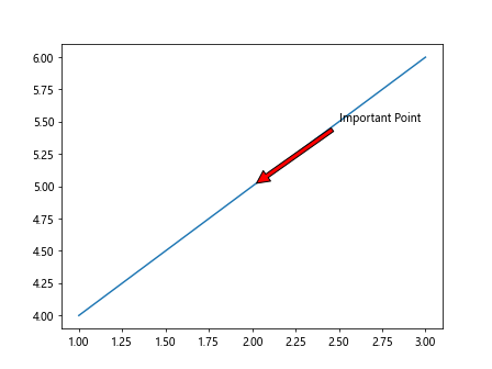
In this example, we are adding the annotation “Important Point” to the point (2, 5) on the plot.

Customizing Annotations

We can customize the appearance of annotations by specifying additional properties in the annotate method. Here are some common properties that can be customized:
– fontsize: The font size of the text.
– color: The color of the text.
– arrowstyle: The style of the arrow.
– connectionstyle: The style of the connection between the annotation and the point.

Let’s see an example of customizing the appearance of an annotation:

import matplotlib.pyplot as plt

fig, ax = plt.subplots()
ax.plot([1, 2, 3], [4, 5, 6])
ax.annotate('Custom Annotation', xy=(2, 5), xytext=(2.5, 5.5),
            arrowprops=dict(facecolor='green', shrink=0.05),
            fontsize=12, color='blue', arrowstyle='wedge', connectionstyle='arc3,rad=0.5')
plt.show()

In this example, we have customized the font size, color, arrow style, and connection style of the annotation.

Using Annotations with Subplots

Annotations can also be added to subplots in Matplotlib. We can specify the subplot to add the annotation to by passing the Axes object to the annotate method. Here is an example of adding annotations to multiple subplots:

import matplotlib.pyplot as plt

fig, axs = plt.subplots(2)
fig.subplots_adjust(hspace=0.5)

axs[0].plot([1, 2, 3], [4, 5, 6])
axs[0].annotate('Annotation 1', xy=(2, 5), xytext=(2.5, 5.5),
                arrowprops=dict(facecolor='purple', shrink=0.05))

axs[1].plot([3, 2, 1], [6, 5, 4])
axs[1].annotate('Annotation 2', xy=(2, 5), xytext=(1.5, 5.5),
                arrowprops=dict(facecolor='orange', shrink=0.05))
plt.show()

Output:

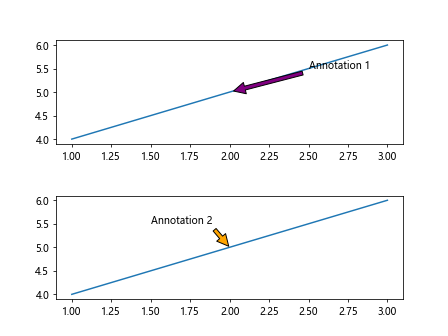
In this example, we have added annotations to two subplots.

Annotations with Custom Arrows

We can create custom arrows for annotations by using the FancyArrowPatch class in Matplotlib. This allows us to define custom shapes for the arrows. Here is an example of creating a custom arrow for an annotation:

import matplotlib.pyplot as plt
import matplotlib.patches as mpatches

fig, ax = plt.subplots()
ax.plot([1, 2, 3], [4, 5, 6])

arrow = mpatches.FancyArrowPatch((1.5, 4.5), (2.5, 5.5),
                                 connectionstyle='arc3,rad=0.5',
                                 arrowstyle='Simple,tail_width=1,head_width=2,head_length=2')
ax.add_patch(arrow)
ax.annotate('Custom Arrow', xy=(2, 5), xytext=(1.5, 4.5), fontsize=12, color='red')
plt.show()

Output:

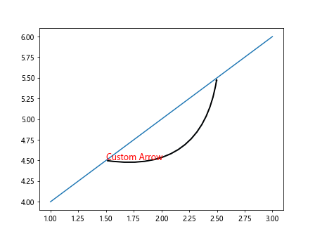
In this example, we have created a custom arrow for the annotation using the FancyArrowPatch class.

Annotations with Arrow Props

The arrowprops argument in the annotate method allows us to customize the properties of the arrow that connects the annotation to the point. We can specify various properties such as the color, arrow style, and connection style. Here is an example of using different arrow properties for annotations:

import matplotlib.pyplot as plt

fig, ax = plt.subplots()
ax.plot([1, 2, 3], [4, 5, 6])

ax.annotate('Arrow Properties 1', xy=(2, 5), xytext=(2.5, 5.5),
            arrowprops=dict(arrowstyle='->', connectionstyle='arc3,rad=0.5',
                            color='purple', linewidth=2, linestyle='--', antialiased=False))

ax.annotate('Arrow Properties 2', xy=(1, 4), xytext=(1.5, 4.5),
            arrowprops=dict(arrowstyle='-[', connectionstyle='arc3,rad=0.2',
                            color='orange', linewidth=2, linestyle=':', antialiased=True))
plt.show()

Output:

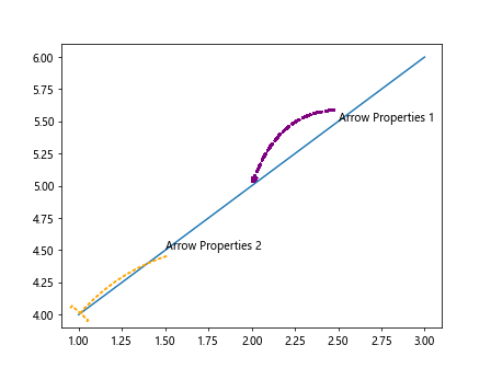
In this example, we have used different arrow properties for two annotations.

Annotations with Text Properties

We can customize the text properties of annotations such as font size, font weight, and text alignment. This allows us to control the appearance of the text in the annotation. Here is an example of using different text properties for annotations:

import matplotlib.pyplot as plt

fig, ax = plt.subplots()
ax.plot([1, 2, 3], [4, 5, 6])

ax.annotate('Text Properties 1', xy=(2, 5), xytext=(2.5, 5.5),
            fontsize=12, color='blue', weight='bold', ha='right', va='bottom')

ax.annotate('Text Properties 2', xy=(1, 4), xytext=(1.5, 4.5),
            fontsize=14, color='green', weight='normal', ha='left', va='top')
plt.show()

Output:

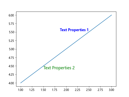
In this example, we have used different text properties for two annotations.

Annotations with Connection Styles

The connectionstyle property in the arrowprops argument allows us to specify the style of the connection between the annotation and the point. We can use different connection styles to create various types of connections. Here is an example of using different connection styles for annotations:

import matplotlib.pyplot as plt

fig, ax = plt.subplots()
ax.plot([1, 2, 3], [4, 5, 6])

ax.annotate('Connection Style 1', xy=(2, 5), xytext=(2.5, 5.5),
            arrowprops=dict(connectionstyle='angle,angleA=0,angleB=90,rad=0.5'))

ax.annotate('Connection Style 2', xy=(1, 4), xytext=(1.5, 4.5),
            arrowprops=dict(connectionstyle='arc3,rad=0.2'))
plt.show()

In this example, we have used different connection styles for two annotations.

Annotations with Bbox Properties

We can add a bounding box around annotations to highlight them. The bbox argument in the annotate method allows us to specify properties for the bounding box such as the color, padding, and transparency. Here is an example of adding a bounding box around an annotation:

import matplotlib.pyplot as plt

fig, ax = plt.subplots()
ax.plot([1, 2, 3], [4, 5, 6])

ax.annotate('Bbox Properties', xy=(2, 5), xytext=(2.5, 5.5),
            arrowprops=dict(facecolor='yellow', shrink=0.05),
            bbox=dict(boxstyle='round,pad=0.5', facecolor='cyan', edgecolor='red', alpha=0.5))
plt.show()

Output:

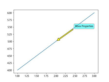
In this example, we have added a bounding box with custom properties around the annotation.

Annotations with Multiple Text Lines

We can add annotations with multiple text lines by using the \n character to separate the lines. This allows us to display additional information in the annotation. Here is an example of adding an annotation with multiple text lines:

import matplotlib.pyplot as plt

fig, ax = plt.subplots()
ax.plot([1, 2, 3], [4, 5, 6])

ax.annotate('Multiple\nLines\nAnnotation', xy=(2, 5), xytext=(2.5, 5.5),
            arrowprops=dict(facecolor='purple', shrink=0.05))
plt.show()

Output:

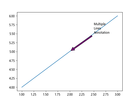
In this example, we have added an annotation with multiple text lines to the plot.

Annotations with LaTeX Math Text

We can use LaTeX math text in annotations to display mathematical equations or symbols. By using LaTeX math mode, we can create complex mathematical expressions in annotations. Here is an example of adding LaTeX math text to an annotation:

import matplotlib.pyplot as plt

fig, ax = plt.subplots()
ax.plot([1, 2, 3], [4, 5, 6])

ax.annotate(r'\frac{a}{b} = c', xy=(2, 5), xytext=(2.5, 5.5),
            arrowprops=dict(facecolor='green', shrink=0.05))
plt.show()

Output:

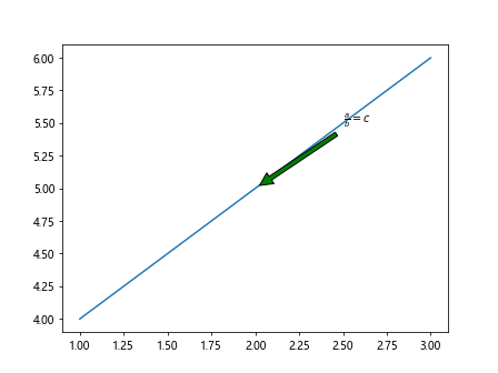
In this example, we have added a mathematical equation using LaTeX math text in the annotation.

Annotations with User Defined Coordinates

We can add annotations with user-defined coordinates by specifying the coordinates as a tuple. This allows us to place annotations at arbitrary points on the plot. Here is an example of adding an annotation with user-defined coordinates:

import matplotlib.pyplot as plt

fig, ax = plt.subplots()
ax.plot([1, 2, 3], [4, 5, 6])

user_coords = (1.8, 4.8)
ax.annotate('User Defined\nCoordinates', xy=(2, 5), xytext=user_coords,
            arrowprops=dict(facecolor='orange', shrink=0.05))
plt.show()

Output:

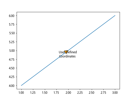
In this example, we have added an annotation at user-defined coordinates on the plot.

Annotations with Relative Coordinates

We can add annotations with relative coordinates by specifying the coordinates as a fraction of the plot size. This allows us to place annotations at specific positions relative to the plot. Here is an example of adding an annotation with relative coordinates:

import matplotlib.pyplot as plt

fig, ax = plt.subplots()
ax.plot([1, 2, 3], [4, 5, 6])

rel_coords = (0.8, 0.8)
ax.annotate('Relative\nCoordinates', xy=(2, 5), xytext=rel_coords,
            arrowprops=dict(facecolor='blue', shrink=0.05))
plt.show()

Output:

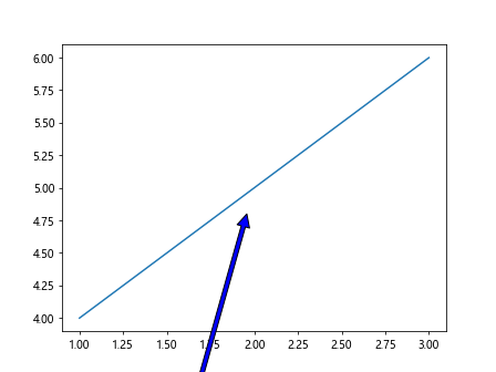
In this example, we have added an annotation at relative coordinates on the plot.

Annotations with Point Annotations

We can add point annotations to highlight specific points on the plot. Point annotations are useful for drawing attention to important data points. Here is an example of adding a point annotation to a plot:

import matplotlib.pyplot as plt

fig, ax = plt.subplots()
ax.plot([1, 2, 3], [4, 5, 6])

for i, j in zip([1, 2, 3], [4, 5, 6]):
    ax.annotate(f'Point ({i},{j})', xy=(i, j), xytext=(i+0.1, j+0.1),
                arrowprops=dict(facecolor='red', shrink=0.05))
plt.show()

Output:

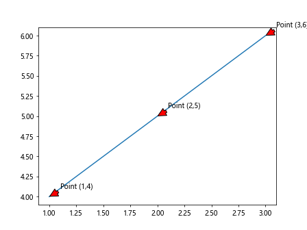
In this example, we have added point annotations to highlight specific data points on the plot.

Annotations with Polar Coordinates

We can add annotations with polar coordinates to plots with a polar projection. Polar coordinates are useful for plotting data on a circular grid. Here is an example of adding an annotation with polar coordinates to a polar plot:

import matplotlib.pyplot as plt
import numpy as np

fig = plt.figure()
ax = fig.add_subplot(111, polar=True)

r = np.array([1, 2, 3])
theta = np.array([np.pi/4, np.pi/2, 3*np.pi/4])
ax.plot(theta, r)

ax.annotate('Polar\nCoordinates', xy=(np.pi/2, 2), xytext=(np.pi/2, 3),
            arrowprops=dict(facecolor='green', shrink=0.05))
plt.show()

Output:

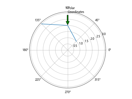
In this example, we have added an annotation with polar coordinates to a polar plot.

Annotations with Categorical Coordinates

We can add annotations with categorical coordinates to plots with categorical axes. Categorical coordinates are useful for annotating categorical data. Here is an example of adding an annotation with categorical coordinates to a plot:

import matplotlib.pyplot as plt

fig, ax = plt.subplots()
x = ['A', 'B', 'C']
y = [3, 5, 2]
ax.bar(x, y)

for i, j in zip(x, y):
    ax.annotate(f'{i}:{j}', xy=(i, j), xytext=(i, j+0.5),
                arrowprops=dict(facecolor='orange', shrink=0.05))
plt.show()

Output:

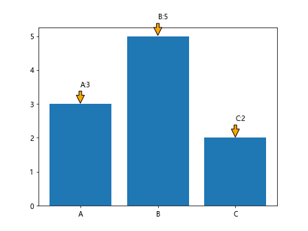
In this example, we have added annotations with categorical coordinates to a bar plot.

Ax Annotate in Matplotlib Conclusion

In this article, we have explored how to use the annotate method in Matplotlib to add annotations to plots. We have covered various aspects of annotations such as customizing annotations, using annotations with subplots, creating custom arrows, and adding annotations with different properties. By mastering the annotate method, you can effectively enhance your plots with annotations and provide additional context to your data. Experiment with the examples provided in this article to create visually appealing and informative plots with annotations in Matplotlib.