How to Master Matplotlib Markers Size: A Comprehensive Guide

How to Master Matplotlib Markers Size: A Comprehensive Guide

Matplotlib markers size is a crucial aspect of data visualization in Python. Understanding how to manipulate marker sizes in Matplotlib can significantly enhance the clarity and impact of your plots. This comprehensive guide will delve deep into the world of Matplotlib markers size, providing you with the knowledge and tools to create stunning visualizations.

Introduction to Matplotlib Markers Size

Matplotlib is a powerful plotting library in Python, and one of its key features is the ability to customize markers. Markers are symbols used to represent data points on a plot, and their size can convey additional information or simply improve the visual appeal of your graphs. The size of these markers can be adjusted using various methods in Matplotlib, allowing for greater flexibility and expressiveness in your data representations.

Let’s start with a basic example of how to set marker size in Matplotlib:

import matplotlib.pyplot as plt

x = [1, 2, 3, 4, 5]
y = [2, 4, 6, 8, 10]

plt.plot(x, y, marker='o', markersize=10, label='how2matplotlib.com')
plt.title('Basic Matplotlib Markers Size Example')
plt.legend()
plt.show()

Output:

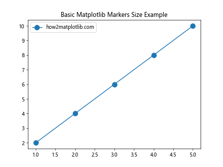
In this example, we set the marker size to 10 using the markersize parameter. This is one of the simplest ways to control Matplotlib markers size.

Understanding Marker Size Units in Matplotlib

When working with Matplotlib markers size, it’s essential to understand the units used. By default, marker sizes are specified in points. One point is approximately 1/72 of an inch. However, Matplotlib also allows you to use other units, such as inches or pixels, depending on your needs.

Here’s an example demonstrating the use of different units for Matplotlib markers size:

import matplotlib.pyplot as plt

x = [1, 2, 3, 4]
y = [1, 2, 3, 4]

fig, (ax1, ax2) = plt.subplots(1, 2, figsize=(10, 5))

ax1.plot(x, y, marker='o', markersize=10, label='Points')
ax1.set_title('Marker Size in Points')

ax2.plot(x, y, marker='o', markersize=0.2, label='Inches')
ax2.set_title('Marker Size in Inches')

for ax in (ax1, ax2):
    ax.legend()
    ax.text(2, 2, 'how2matplotlib.com', fontsize=12)

plt.tight_layout()
plt.show()

Output:

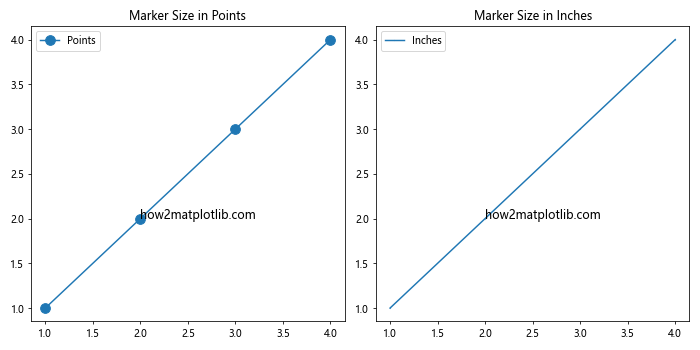
In this example, we create two subplots. The first uses the default point units, while the second uses inches by setting markersize=0.2.

Varying Marker Sizes Based on Data

One of the most powerful applications of Matplotlib markers size is to represent an additional dimension of your data. By varying the size of markers based on a data variable, you can convey more information in a single plot.

Here’s an example of how to achieve this:

import matplotlib.pyplot as plt
import numpy as np

x = np.random.rand(50)
y = np.random.rand(50)
sizes = np.random.rand(50) * 1000  # Varying sizes

plt.scatter(x, y, s=sizes, alpha=0.5, label='Data Points')
plt.title('Varying Matplotlib Markers Size')
plt.xlabel('X-axis')
plt.ylabel('Y-axis')
plt.legend()
plt.text(0.5, 0.5, 'how2matplotlib.com', fontsize=12)
plt.show()

Output:

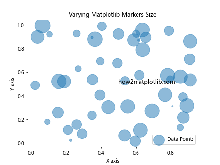
In this scatter plot, the size of each marker is determined by the sizes array, which contains random values. The s parameter in plt.scatter() is used to set these varying sizes.

Setting Marker Size in Line Plots

While scatter plots are commonly used for varying marker sizes, you can also adjust marker sizes in line plots. This can be particularly useful when you want to emphasize certain data points along a line.

Here’s how you can do this:

import matplotlib.pyplot as plt
import numpy as np

x = np.linspace(0, 10, 10)
y = np.sin(x)
sizes = np.linspace(20, 200, 10)  # Increasing sizes

plt.plot(x, y, marker='o', label='Sine Wave')
plt.scatter(x, y, s=sizes, c='red', label='Emphasized Points')
plt.title('Line Plot with Varying Matplotlib Markers Size')
plt.xlabel('X-axis')
plt.ylabel('Y-axis')
plt.legend()
plt.text(5, 0, 'how2matplotlib.com', fontsize=12)
plt.show()

Output:

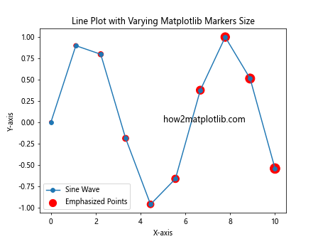
In this example, we combine a line plot with a scatter plot. The scatter plot uses varying marker sizes to emphasize certain points along the sine wave.

Using Marker Size to Represent Categorical Data

Matplotlib markers size can also be used to represent categorical data. By assigning different sizes to different categories, you can create visually distinctive plots that clearly show category differences.

Here’s an example:

import matplotlib.pyplot as plt
import numpy as np

categories = ['A', 'B', 'C', 'D']
values = [15, 25, 35, 45]
sizes = [100, 200, 300, 400]

plt.scatter(categories, values, s=sizes, alpha=0.7)
plt.title('Categorical Data with Varying Matplotlib Markers Size')
plt.xlabel('Categories')
plt.ylabel('Values')
for i, txt in enumerate(categories):
    plt.annotate(f'{txt}: {values[i]}', (i, values[i]), xytext=(5,5), textcoords='offset points')
plt.text(1.5, 30, 'how2matplotlib.com', fontsize=12)
plt.show()

Output:

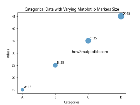
In this example, each category is represented by a marker of a different size, making it easy to distinguish between them visually.

Customizing Marker Size Legends

When using varying marker sizes, it’s often helpful to include a legend that explains what the different sizes represent. Matplotlib provides ways to create custom legends for marker sizes.

Here’s an example of how to create a custom legend for marker sizes:

import matplotlib.pyplot as plt
import numpy as np

x = np.random.rand(50)
y = np.random.rand(50)
sizes = np.random.rand(50) * 1000

scatter = plt.scatter(x, y, s=sizes, alpha=0.5)
plt.title('Scatter Plot with Matplotlib Markers Size Legend')

# Creating legend elements
legend_elements = [plt.scatter([], [], s=size, label=f'Size {size}') for size in [100, 500, 1000]]

plt.legend(handles=legend_elements, title='Marker Sizes')
plt.text(0.5, 0.5, 'how2matplotlib.com', fontsize=12)
plt.show()

Output:

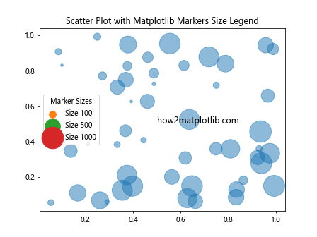
This example creates a custom legend that shows three different marker sizes and their corresponding labels.

Adjusting Marker Size for Multiple Datasets

When plotting multiple datasets on the same graph, you may want to use different marker sizes to distinguish between them. This can be particularly useful when dealing with datasets of varying importance or scale.

Here’s how you can achieve this:

import matplotlib.pyplot as plt
import numpy as np

x = np.linspace(0, 10, 50)
y1 = np.sin(x)
y2 = np.cos(x)

plt.plot(x, y1, marker='o', markersize=5, label='Sin')
plt.plot(x, y2, marker='s', markersize=10, label='Cos')
plt.title('Multiple Datasets with Different Matplotlib Markers Size')
plt.xlabel('X-axis')
plt.ylabel('Y-axis')
plt.legend()
plt.text(5, 0, 'how2matplotlib.com', fontsize=12)
plt.show()

Output:

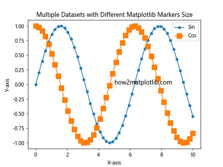
In this example, we use different marker sizes (and shapes) for the sine and cosine functions to make them easily distinguishable.

Marker Size in 3D Plots

Matplotlib markers size can also be manipulated in 3D plots, adding an extra dimension to your visualizations. This can be particularly useful for representing complex datasets.

Here’s an example of how to use varying marker sizes in a 3D scatter plot:

import matplotlib.pyplot as plt
import numpy as np

fig = plt.figure(figsize=(10, 8))
ax = fig.add_subplot(111, projection='3d')

n = 100
xs = np.random.rand(n)
ys = np.random.rand(n)
zs = np.random.rand(n)
sizes = np.random.rand(n) * 100

scatter = ax.scatter(xs, ys, zs, s=sizes, c=sizes, cmap='viridis')

ax.set_xlabel('X Label')
ax.set_ylabel('Y Label')
ax.set_zlabel('Z Label')
ax.set_title('3D Scatter Plot with Varying Matplotlib Markers Size')

plt.colorbar(scatter, label='Size')
ax.text(0.5, 0.5, 0.5, 'how2matplotlib.com', fontsize=12)
plt.show()

Output:

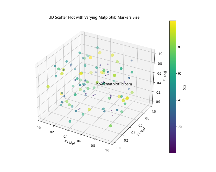
In this 3D scatter plot, we use marker size to represent an additional dimension of the data, with a colorbar to indicate the size scale.

Animating Marker Size Changes

Matplotlib also allows for the animation of marker sizes, which can be useful for showing how data changes over time or through iterations.

Here’s a simple example of how to create an animation with changing marker sizes:

import matplotlib.pyplot as plt
import matplotlib.animation as animation
import numpy as np

fig, ax = plt.subplots()

x = np.linspace(0, 2*np.pi, 100)
y = np.sin(x)

line, = ax.plot(x, y, 'o')

def animate(i):
    size = 5 + 5 * np.sin(i * 0.1)
    line.set_markersize(size)
    return line,

ani = animation.FuncAnimation(fig, animate, frames=200, interval=50, blit=True)
plt.title('Animated Matplotlib Markers Size')
plt.text(np.pi, 0, 'how2matplotlib.com', fontsize=12)
plt.show()

Output:

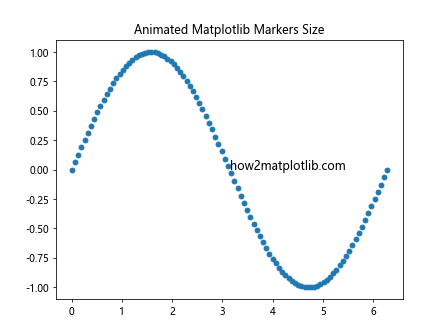
This animation shows markers changing size sinusoidally over time.

Marker Size and Data Density

When dealing with dense datasets, adjusting marker size can help prevent overcrowding and make your plots more readable. Smaller markers can be used for dense regions, while larger markers can be used for sparse regions.

Here’s an example demonstrating this concept:

import matplotlib.pyplot as plt
import numpy as np

np.random.seed(42)
x = np.concatenate([np.random.normal(0, 1, 1000), np.random.normal(5, 1, 100)])
y = np.concatenate([np.random.normal(0, 1, 1000), np.random.normal(5, 1, 100)])

density = plt.hist2d(x, y, bins=20)[0]
plt.clf()  # Clear the histogram

sizes = 1000 / (density + 10)  # Inverse relationship with density

plt.scatter(x, y, s=sizes.flatten()[np.searchsorted(np.sort(x), x)], alpha=0.5)
plt.title('Matplotlib Markers Size Adjusted for Data Density')
plt.xlabel('X-axis')
plt.ylabel('Y-axis')
plt.text(2.5, 2.5, 'how2matplotlib.com', fontsize=12)
plt.show()

In this example, we adjust the marker size based on the local density of points, with smaller markers in dense regions and larger markers in sparse regions.

Marker Size and Color Mapping

Combining marker size variations with color mapping can create highly informative visualizations. This technique allows you to represent three dimensions of data in a 2D plot.

Here’s an example:

import matplotlib.pyplot as plt
import numpy as np

x = np.random.rand(50)
y = np.random.rand(50)
sizes = np.random.rand(50) * 1000
colors = np.random.rand(50)

plt.scatter(x, y, s=sizes, c=colors, alpha=0.5, cmap='viridis')
plt.colorbar(label='Color Value')
plt.title('Matplotlib Markers Size and Color Mapping')
plt.xlabel('X-axis')
plt.ylabel('Y-axis')
plt.text(0.5, 0.5, 'how2matplotlib.com', fontsize=12)
plt.show()

Output:

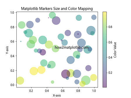
In this scatter plot, the size of each marker represents one dimension of the data, while its color represents another.

Marker Size in Polar Plots

Matplotlib markers size can also be adjusted in polar plots, which can be particularly useful for circular data representations.

Here’s an example of a polar plot with varying marker sizes:

import matplotlib.pyplot as plt
import numpy as np

theta = np.linspace(0, 2*np.pi, 20)
r = 10 * np.random.rand(20)
sizes = r * 50  # Size proportional to radius

fig, ax = plt.subplots(subplot_kw=dict(projection='polar'))
ax.scatter(theta, r, s=sizes, c=theta, cmap='hsv', alpha=0.75)

ax.set_title('Polar Plot with Varying Matplotlib Markers Size')
plt.text(np.pi/2, 5, 'how2matplotlib.com', fontsize=12)
plt.show()

Output:

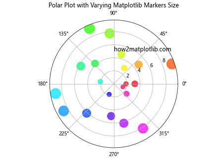
In this polar plot, the size of each marker is proportional to its radial distance from the center.

Marker Size in Subplots

When working with subplots, you may want to adjust marker sizes differently for each subplot. This can help emphasize different aspects of your data across multiple plots.

Here’s an example:

import matplotlib.pyplot as plt
import numpy as np

fig, (ax1, ax2) = plt.subplots(1, 2, figsize=(12, 5))

x = np.linspace(0, 10, 50)
y1 = np.sin(x)
y2 = np.cos(x)

ax1.scatter(x, y1, s=x*10, label='Sin')
ax1.set_title('Increasing Matplotlib Markers Size')

ax2.scatter(x, y2, s=(10-x)*10, label='Cos')
ax2.set_title('Decreasing Matplotlib Markers Size')

for ax in (ax1, ax2):
    ax.set_xlabel('X-axis')
    ax.set_ylabel('Y-axis')
    ax.legend()
    ax.text(5, 0, 'how2matplotlib.com', fontsize=10)

plt.tight_layout()
plt.show()

Output:

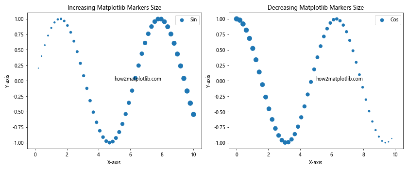
In this example, we create two subplots with different marker size patterns: one increasing and one decreasing along the x-axis.

Marker Size and Error Bars

When working with data that includes uncertainty, you can combine marker size adjustments with error bars to create more informative plots.

Here’s an example:

import matplotlib.pyplot as plt
import numpy as np

x = np.linspace(0, 10, 10)
y = np.sin(x)
error = np.random.rand(10) * 0.2
sizes = np.linspace(20, 200, 10)

plt.errorbar(x, y, yerr=error, fmt='o', capsize=5, capthick=2, ecolor='gray', markersize=10)
plt.scatter(x, y, s=sizes, c='red', zorder=2)
plt.title('Matplotlib Markers Size with Error Bars')
plt.xlabel('X-axis')
plt.ylabel('Y-axis')
plt.text(5, 0, 'how2matplotlib.com', fontsize=12)
plt.show()

Output:

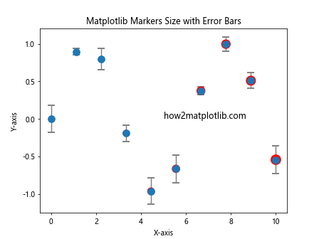
In this plot, we combine error bars with markers of varying sizes to represent both the uncertainty in the data and an additional dimensionof information.

Marker Size in Heatmaps

While heatmaps typically use color to represent data values, incorporating marker size can add an extra dimension to your visualization. This can be particularly useful when you want to emphasize certain data points within the heatmap.

Here’s an example of how to create a heatmap with varying marker sizes:

import matplotlib.pyplot as plt
import numpy as np

data = np.random.rand(10, 10)
x, y = np.meshgrid(np.arange(10), np.arange(10))
sizes = data * 500

plt.imshow(data, cmap='viridis')
plt.scatter(x, y, s=sizes, c='white', alpha=0.5)
plt.colorbar(label='Data Value')
plt.title('Heatmap with Varying Matplotlib Markers Size')
plt.text(4, 4, 'how2matplotlib.com', fontsize=12, color='white')
plt.show()

Output:

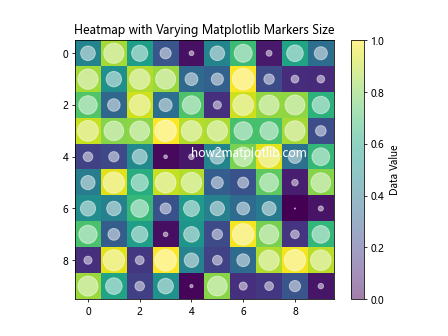
In this example, we overlay a scatter plot with varying marker sizes on top of a heatmap, providing two ways to visualize the same data.

Marker Size in Network Graphs

When visualizing network graphs, adjusting marker sizes can help emphasize important nodes or represent node attributes. Matplotlib can be used in conjunction with network libraries like NetworkX to create these visualizations.

Here’s an example:

import matplotlib.pyplot as plt
import networkx as nx
import numpy as np

G = nx.random_geometric_graph(20, 0.3)
pos = nx.spring_layout(G)

degrees = dict(nx.degree(G))
node_sizes = [v * 100 for v in degrees.values()]

nx.draw(G, pos, node_size=node_sizes, with_labels=True, node_color='lightblue')
plt.title('Network Graph with Varying Matplotlib Markers Size')
plt.text(0.5, 0.5, 'how2matplotlib.com', fontsize=12, transform=plt.gca().transAxes)
plt.show()

Output:

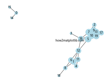
In this network graph, the size of each node is proportional to its degree (number of connections).

Marker Size and Transparency

Combining marker size adjustments with transparency can be particularly useful when dealing with overlapping data points. This technique allows you to see the density of data points in crowded areas.

Here’s an example:

import matplotlib.pyplot as plt
import numpy as np

x = np.random.normal(0, 1, 1000)
y = np.random.normal(0, 1, 1000)
sizes = np.random.rand(1000) * 100

plt.scatter(x, y, s=sizes, alpha=0.5)
plt.title('Scatter Plot with Varying Matplotlib Markers Size and Transparency')
plt.xlabel('X-axis')
plt.ylabel('Y-axis')
plt.text(0, 0, 'how2matplotlib.com', fontsize=12)
plt.show()

Output:

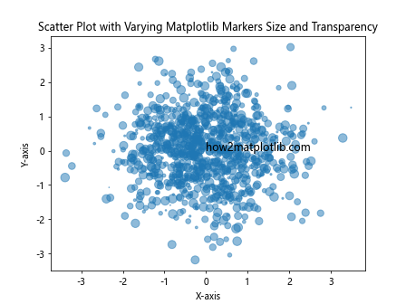
In this scatter plot, larger markers are more transparent, allowing smaller markers behind them to be visible.

Marker Size in Time Series Data

When working with time series data, adjusting marker sizes can help highlight trends or important events over time.

Here’s an example:

import matplotlib.pyplot as plt
import pandas as pd
import numpy as np

dates = pd.date_range(start='2023-01-01', end='2023-12-31', freq='D')
values = np.cumsum(np.random.randn(len(dates)))
sizes = np.abs(values) * 10

plt.figure(figsize=(12, 6))
plt.scatter(dates, values, s=sizes, alpha=0.6)
plt.plot(dates, values, alpha=0.3)
plt.title('Time Series with Varying Matplotlib Markers Size')
plt.xlabel('Date')
plt.ylabel('Value')
plt.text(dates[len(dates)//2], 0, 'how2matplotlib.com', fontsize=12)
plt.show()

Output:

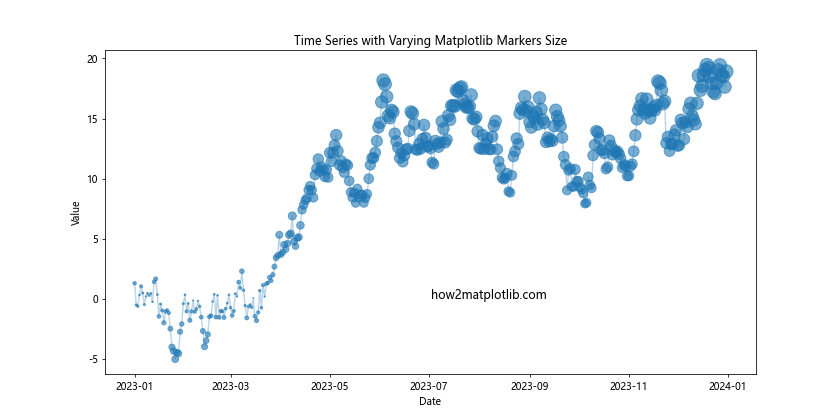
In this time series plot, the size of each marker is proportional to the absolute value of the data point, emphasizing larger values.

Matplotlib markers size Conclusion

Mastering Matplotlib markers size is a powerful skill that can significantly enhance your data visualizations. By adjusting marker sizes, you can add an extra dimension to your plots, emphasize important data points, and create more informative and visually appealing graphs.

Throughout this comprehensive guide, we’ve explored various aspects of Matplotlib markers size, including:

1. Basic marker size adjustment
2. Understanding size units
3. Varying sizes based on data
4. Using size in different types of plots (scatter, line, 3D, polar)
5. Creating custom legends for marker sizes
6. Animating marker size changes
7. Adjusting size for data density
8. Combining size with color mapping
9. Using size in subplots and with error bars
10. Incorporating size in heatmaps and network graphs
11. Combining size adjustments with transparency
12. Utilizing marker size in time series data

By mastering these techniques, you’ll be able to create more sophisticated and informative visualizations that effectively communicate your data insights.

Remember, the key to effective data visualization is not just making your plots look good, but ensuring they convey information clearly and efficiently. Thoughtful use of Matplotlib markers size can help you achieve this goal, allowing you to create plots that are both visually striking and rich in information.

As you continue to work with Matplotlib, experiment with different marker sizes and combinations of techniques to find the best way to represent your specific data. With practice, you’ll develop an intuition for when and how to adjust marker sizes to create the most effective visualizations for your needs.

Matplotlib’s flexibility and extensive feature set make it a powerful tool for data visualization in Python. By mastering Matplotlib markers size, you’re adding a valuable skill to your data visualization toolkit, enabling you to create more nuanced and informative plots that can help you and others better understand and interpret complex datasets.

Whether you’re working in data science, scientific research, finance, or any other field that requires data visualization, the ability to effectively use Matplotlib markers size will serve you well. It’s a skill that can help you stand out in your field and communicate your findings more effectively to both technical and non-technical audiences.