Comprehensive Guide to 3D Surface Plotting in Python using Matplotlib

Comprehensive Guide to 3D Surface Plotting in Python using Matplotlib

3D Surface plotting in Python using Matplotlib is a powerful technique for visualizing three-dimensional data. This article will explore various aspects of creating 3D surface plots with Matplotlib, providing detailed explanations and examples to help you master this essential data visualization skill.

Introduction to 3D Surface Plotting in Python using Matplotlib

3D Surface plotting in Python using Matplotlib allows you to represent three-dimensional data in a visually appealing and informative way. These plots are particularly useful for displaying mathematical functions, terrain data, or any dataset with three variables. Matplotlib, a popular plotting library in Python, provides robust tools for creating 3D surface plots with ease.

To get started with 3D surface plotting in Python using Matplotlib, you’ll need to import the necessary modules:

import numpy as np
import matplotlib.pyplot as plt
from mpl_toolkits.mplot3d import Axes3D

# Create a figure and a 3D axis
fig = plt.figure(figsize=(10, 8))
ax = fig.add_subplot(111, projection='3d')

# Generate sample data
x = np.linspace(-5, 5, 100)
y = np.linspace(-5, 5, 100)
X, Y = np.meshgrid(x, y)
Z = np.sin(np.sqrt(X**2 + Y**2))

# Create the surface plot
surf = ax.plot_surface(X, Y, Z, cmap='viridis')

# Add a color bar
fig.colorbar(surf)

# Set labels and title
ax.set_xlabel('X-axis')
ax.set_ylabel('Y-axis')
ax.set_zlabel('Z-axis')
ax.set_title('3D Surface Plot - how2matplotlib.com')

plt.show()

Output:

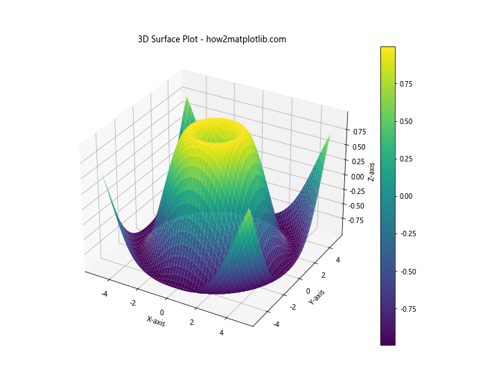
This example demonstrates the basic structure of creating a 3D surface plot using Matplotlib. We’ll dive deeper into each aspect of 3D surface plotting in the following sections.

Understanding the Basics of 3D Surface Plotting in Python using Matplotlib

Before we delve into more advanced techniques, it’s essential to understand the fundamental components of 3D surface plotting in Python using Matplotlib:

1. Data preparation: You need to create a grid of X and Y values and calculate the corresponding Z values.
2. Creating the plot: Use the plot_surface() function to generate the 3D surface.
3. Customizing the appearance: Adjust colors, labels, and other visual elements to enhance the plot.

Let’s explore these components in more detail:

import numpy as np
import matplotlib.pyplot as plt
from mpl_toolkits.mplot3d import Axes3D

# Data preparation
x = np.linspace(-5, 5, 50)
y = np.linspace(-5, 5, 50)
X, Y = np.meshgrid(x, y)
Z = X**2 + Y**2

# Creating the plot
fig = plt.figure(figsize=(10, 8))
ax = fig.add_subplot(111, projection='3d')
surf = ax.plot_surface(X, Y, Z, cmap='coolwarm')

# Customizing the appearance
ax.set_xlabel('X-axis')
ax.set_ylabel('Y-axis')
ax.set_zlabel('Z-axis')
ax.set_title('Basic 3D Surface Plot - how2matplotlib.com')
fig.colorbar(surf, shrink=0.5, aspect=5)

plt.show()

Output:

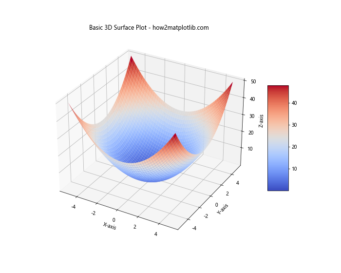
This example illustrates the basic steps in creating a 3D surface plot. We’ll explore each of these steps in more detail throughout the article.

Advanced Techniques for 3D Surface Plotting in Python using Matplotlib

Now that we’ve covered the basics, let’s explore some advanced techniques for 3D surface plotting in Python using Matplotlib:

Customizing Color Maps in 3D Surface Plotting

Color maps play a crucial role in enhancing the visual appeal and interpretability of 3D surface plots. Matplotlib offers a wide range of color maps that you can use to represent your data effectively:

import numpy as np
import matplotlib.pyplot as plt
from mpl_toolkits.mplot3d import Axes3D

# Generate data
x = np.linspace(-5, 5, 100)
y = np.linspace(-5, 5, 100)
X, Y = np.meshgrid(x, y)
Z = np.sin(np.sqrt(X**2 + Y**2))

# Create subplots
fig, (ax1, ax2) = plt.subplots(1, 2, figsize=(15, 6), subplot_kw={'projection': '3d'})

# Plot with 'viridis' colormap
surf1 = ax1.plot_surface(X, Y, Z, cmap='viridis')
ax1.set_title('Viridis Colormap - how2matplotlib.com')

# Plot with 'plasma' colormap
surf2 = ax2.plot_surface(X, Y, Z, cmap='plasma')
ax2.set_title('Plasma Colormap - how2matplotlib.com')

# Add colorbars
fig.colorbar(surf1, ax=ax1, shrink=0.5, aspect=5)
fig.colorbar(surf2, ax=ax2, shrink=0.5, aspect=5)

plt.tight_layout()
plt.show()

Output:

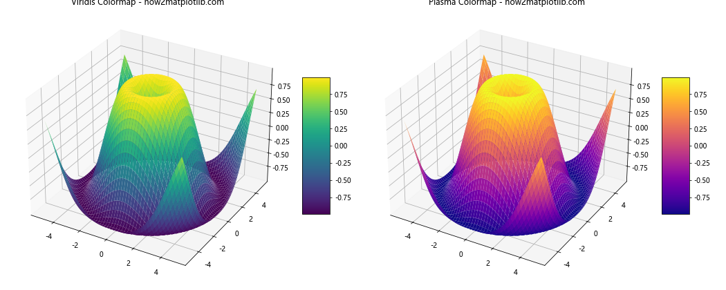
This example demonstrates how to use different color maps for 3D surface plotting in Python using Matplotlib. Experiment with various color maps to find the one that best represents your data.

Adding Contour Plots to 3D Surface Plots

Combining contour plots with 3D surface plots can provide additional insights into your data. Here’s how you can add contour plots to your 3D surface plot:

import numpy as np
import matplotlib.pyplot as plt
from mpl_toolkits.mplot3d import Axes3D

# Generate data
x = np.linspace(-5, 5, 100)
y = np.linspace(-5, 5, 100)
X, Y = np.meshgrid(x, y)
Z = np.sin(X) * np.cos(Y)

# Create the plot
fig = plt.figure(figsize=(10, 8))
ax = fig.add_subplot(111, projection='3d')

# Plot the surface
surf = ax.plot_surface(X, Y, Z, cmap='viridis', alpha=0.8)

# Add contour plot
contour = ax.contour(X, Y, Z, zdir='z', offset=-2, cmap='coolwarm')

# Customize the plot
ax.set_zlim(-2, 2)
ax.set_title('3D Surface with Contour Plot - how2matplotlib.com')
fig.colorbar(surf, shrink=0.5, aspect=5)

plt.show()

Output:

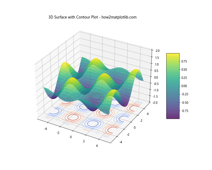
This example shows how to add a contour plot to the base of a 3D surface plot, providing a 2D representation of the data alongside the 3D visualization.

Adjusting View Angle and Perspective in 3D Surface Plotting

The view angle and perspective of your 3D surface plot can significantly impact how the data is perceived. Matplotlib allows you to adjust these parameters easily:

import numpy as np
import matplotlib.pyplot as plt
from mpl_toolkits.mplot3d import Axes3D

# Generate data
x = np.linspace(-5, 5, 100)
y = np.linspace(-5, 5, 100)
X, Y = np.meshgrid(x, y)
Z = np.sin(np.sqrt(X**2 + Y**2))

# Create subplots
fig, (ax1, ax2) = plt.subplots(1, 2, figsize=(15, 6), subplot_kw={'projection': '3d'})

# Plot with default view
surf1 = ax1.plot_surface(X, Y, Z, cmap='viridis')
ax1.set_title('Default View - how2matplotlib.com')

# Plot with adjusted view
surf2 = ax2.plot_surface(X, Y, Z, cmap='viridis')
ax2.view_init(elev=20, azim=45)
ax2.set_title('Adjusted View - how2matplotlib.com')

plt.tight_layout()
plt.show()

Output:

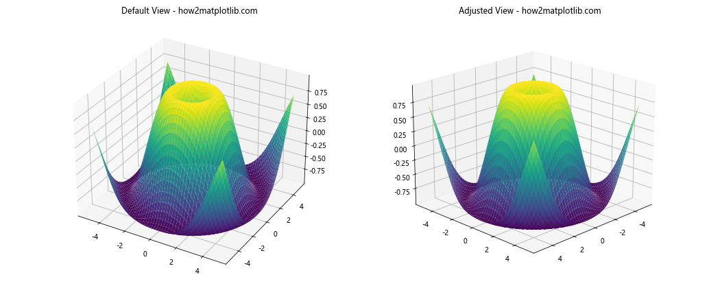
This example demonstrates how to adjust the viewing angle of a 3D surface plot using the view_init() function.

Advanced Data Representation in 3D Surface Plotting using Matplotlib

3D surface plotting in Python using Matplotlib offers various ways to represent complex data. Let’s explore some advanced techniques:

Representing Multiple Datasets in a Single 3D Surface Plot

Sometimes, you may need to compare multiple datasets in a single 3D surface plot. Here’s how you can achieve this:

import numpy as np
import matplotlib.pyplot as plt
from mpl_toolkits.mplot3d import Axes3D

# Generate data
x = np.linspace(-5, 5, 100)
y = np.linspace(-5, 5, 100)
X, Y = np.meshgrid(x, y)
Z1 = np.sin(np.sqrt(X**2 + Y**2))
Z2 = np.cos(np.sqrt(X**2 + Y**2))

# Create the plot
fig = plt.figure(figsize=(12, 8))
ax = fig.add_subplot(111, projection='3d')

# Plot multiple surfaces
surf1 = ax.plot_surface(X, Y, Z1, cmap='viridis', alpha=0.7)
surf2 = ax.plot_surface(X, Y, Z2, cmap='plasma', alpha=0.7)

# Customize the plot
ax.set_title('Multiple Datasets in 3D Surface Plot - how2matplotlib.com')
fig.colorbar(surf1, shrink=0.5, aspect=5, label='Dataset 1')
fig.colorbar(surf2, shrink=0.5, aspect=5, label='Dataset 2')

plt.show()

Output:

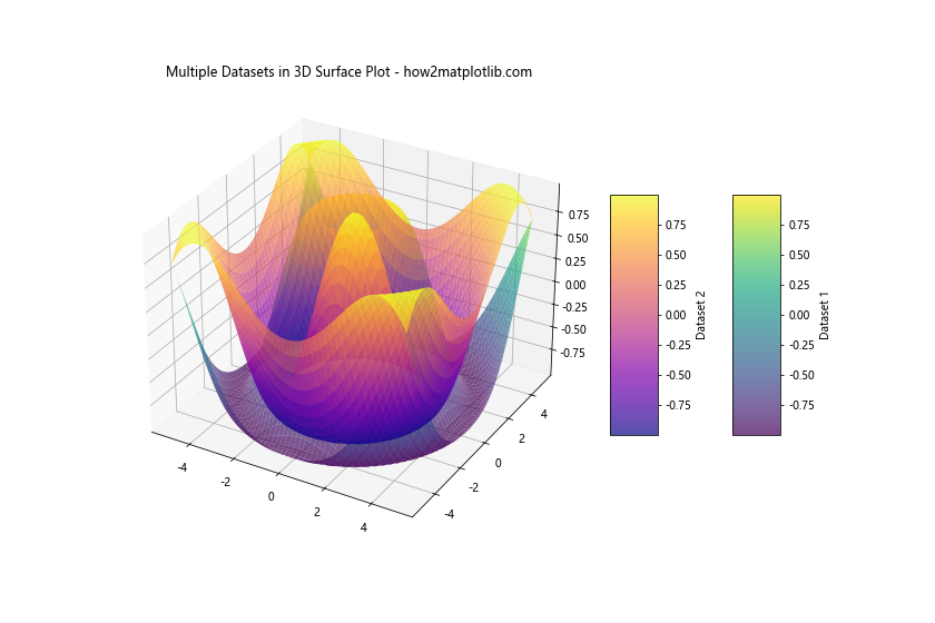
This example shows how to plot two different datasets on the same 3D surface plot, using different color maps and transparency levels to distinguish between them.

Creating Animated 3D Surface Plots

Animated 3D surface plots can be particularly useful for visualizing how data changes over time or with respect to a parameter. Here’s an example of how to create an animated 3D surface plot:

import numpy as np
import matplotlib.pyplot as plt
from mpl_toolkits.mplot3d import Axes3D
from matplotlib.animation import FuncAnimation

# Generate initial data
x = np.linspace(-5, 5, 50)
y = np.linspace(-5, 5, 50)
X, Y = np.meshgrid(x, y)

# Create the plot
fig = plt.figure(figsize=(10, 8))
ax = fig.add_subplot(111, projection='3d')

# Initialize the surface plot
Z = np.sin(np.sqrt(X**2 + Y**2))
surf = ax.plot_surface(X, Y, Z, cmap='viridis')

# Update function for animation
def update(frame):
    ax.clear()
    Z = np.sin(np.sqrt(X**2 + Y**2) + frame / 10)
    surf = ax.plot_surface(X, Y, Z, cmap='viridis')
    ax.set_title(f'Animated 3D Surface Plot - Frame {frame} - how2matplotlib.com')
    return surf,

# Create the animation
anim = FuncAnimation(fig, update, frames=100, interval=50, blit=False)

plt.show()

Output:

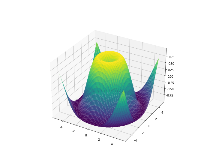
This example creates an animated 3D surface plot where the surface changes over time. Note that to save this animation, you would need to use additional libraries like ffmpeg.

Optimizing 3D Surface Plots in Python using Matplotlib

When working with large datasets or complex visualizations, optimizing your 3D surface plots becomes crucial. Here are some techniques to improve performance and visual clarity:

Adjusting Surface Plot Properties for Better Visualization

Fine-tuning the properties of your 3D surface plot can greatly enhance its visual appeal and readability:

import numpy as np
import matplotlib.pyplot as plt
from mpl_toolkits.mplot3d import Axes3D

# Generate data
x = np.linspace(-5, 5, 100)
y = np.linspace(-5, 5, 100)
X, Y = np.meshgrid(x, y)
Z = np.sin(np.sqrt(X**2 + Y**2))

# Create the plot
fig = plt.figure(figsize=(12, 8))
ax = fig.add_subplot(111, projection='3d')

# Plot the surface with customized properties
surf = ax.plot_surface(X, Y, Z, cmap='viridis',
                       linewidth=0, antialiased=False, alpha=0.8)

# Customize the plot
ax.set_title('Optimized 3D Surface Plot - how2matplotlib.com')
ax.set_xlabel('X-axis')
ax.set_ylabel('Y-axis')
ax.set_zlabel('Z-axis')

# Add a color bar
fig.colorbar(surf, shrink=0.5, aspect=5)

# Adjust the viewing angle
ax.view_init(elev=30, azim=45)

plt.show()

Output:

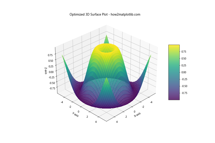
This example shows how to adjust various properties of the surface plot, such as linewidth, antialiasing, and transparency, to create a more visually appealing result.

Advanced Customization Techniques for 3D Surface Plotting in Python using Matplotlib

Matplotlib offers a wide range of customization options for 3D surface plotting. Let’s explore some advanced techniques to make your plots stand out:

Adding Text and Annotations to 3D Surface Plots

Adding text and annotations to your 3D surface plots can provide additional context and highlight important features:

import numpy as np
import matplotlib.pyplot as plt
from mpl_toolkits.mplot3d import Axes3D

# Generate data
x = np.linspace(-5, 5, 100)
y = np.linspace(-5, 5, 100)
X, Y = np.meshgrid(x, y)
Z = np.sin(np.sqrt(X**2 + Y**2))

# Create the plot
fig = plt.figure(figsize=(12, 8))
ax = fig.add_subplot(111, projection='3d')

# Plot the surface
surf = ax.plot_surface(X, Y, Z, cmap='viridis')

# Add text and annotations
ax.text(0, 0, 1, "Peak", color='red', fontsize=12)
ax.text(4, 4, -0.5, "Valley", color='blue', fontsize=12)

# Add an arrow annotation
ax.quiver(0, 0, 0, 0, 0, 1, color='red', length=1, arrow_length_ratio=0.1)

# Customize the plot
ax.set_title('3D Surface Plot with Annotations - how2matplotlib.com')
fig.colorbar(surf, shrink=0.5, aspect=5)

plt.show()

Output:

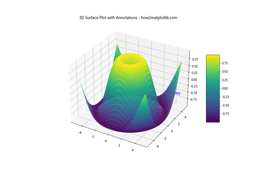
This example demonstrates how to add text labels and arrow annotations to specific points on your 3D surface plot.

Customizing Axis Properties in 3D Surface Plots

Customizing axis properties can greatly enhance the readability and aesthetics of your 3D surface plots:

import numpy as np
import matplotlib.pyplot as plt
from mpl_toolkits.mplot3d import Axes3D

# Generate data
x = np.linspace(-5, 5, 100)
y = np.linspace(-5, 5, 100)
X, Y = np.meshgrid(x, y)
Z = np.sin(np.sqrt(X**2 + Y**2))

# Create the plot
fig = plt.figure(figsize=(12, 8))
ax = fig.add_subplot(111, projection='3d')

# Plot the surface
surf = ax.plot_surface(X, Y, Z, cmap='viridis')

# Customize axis properties
ax.set_xlabel('X-axis', fontsize=12, fontweight='bold')
ax.set_ylabel('Y-axis', fontsize=12, fontweight='bold')
ax.set_zlabel('Z-axis', fontsize=12, fontweight='bold')
ax.set_title('Customized Axis Properties - how2matplotlib.com', fontsize=14)

# Set axis limits
ax.set_xlim(-6, 6)
ax.set_ylim(-6, 6)
ax.set_zlim(-1.5, 1.5)

# Customize tick labels
ax.set_xticks([-5, 0, 5])
ax.set_yticks([-5, 0, 5])
ax.set_zticks([-1, 0, 1])

# Add a color bar
fig.colorbar(surf, shrink=0.5, aspect=5)

plt.show()

Output:

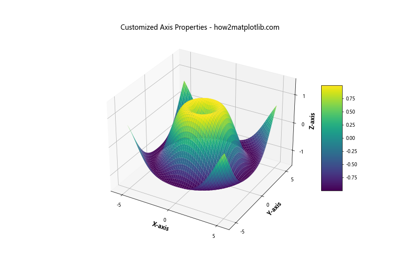
This example shows how to customize various axis properties, including labels, limits, and tick marks, to create a more polished 3D surface plot.

Combining 3D Surface Plots with Other Visualization Techniques

3D surface plotting in Python using Matplotlib can be even more powerful when combined with other visualization techniques. Let’s explore some interesting combinations:

Combining 3D Surface Plots with Scatter Plots

Adding scatter plots to your 3D surface plot can help highlight specific data points or regions of interest:

import numpy as np
import matplotlib.pyplot as plt
from mpl_toolkits.mplot3d import Axes3D

# Generate surface data
x = np.linspace(-5, 5, 100)
y = np.linspace(-5, 5, 100)
X, Y = np.meshgrid(x, y)
Z = np.sin(np.sqrt(X**2 + Y**2))

# Generate scatter data
scatter_x = np.random.uniform(-5, 5, 50)
scatter_y = np.random.uniform(-5, 5, 50)
scatter_z = np.sin(np.sqrt(scatter_x**2 + scatter_y**2)) + np.random.normal(0, 0.1, 50)

# Create the plot
fig = plt.figure(figsize=(12, 8))
ax = fig.add_subplot(111, projection='3d')

# Plot the surface
surf = ax.plot_surface(X, Y, Z, cmap='viridis', alpha=0.8)

# Add scatter plot
ax.scatter(scatter_x, scatter_y, scatter_z, c='red', s=50, label='Data Points')

# Customize the plot
ax.set_xlabel('X-axis')
ax.set_ylabel('Y-axis')
ax.set_zlabel('Z-axis')
ax.set_title('3D Surface Plot with Scatter Points - how2matplotlib.com')
ax.legend()

# Add a color bar
fig.colorbar(surf, shrink=0.5, aspect=5)

plt.show()

Output:

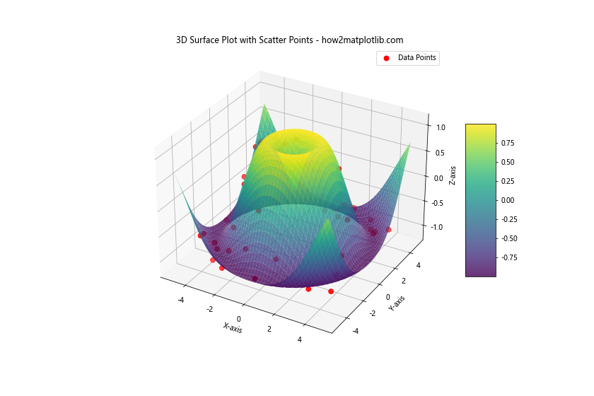
This example demonstrates how to combine a 3D surface plot with a scatter plot to highlight specific data points on the surface.

Handling Common Challenges in 3D Surface Plotting with Matplotlib

While 3D surface plotting in Python using Matplotlib is powerful, you may encounter some challenges. Let’s address some common issues and their solutions:

Dealing with NaN Values in 3D Surface Plots

NaN (Not a Number) values can cause issues in 3D surface plots. Here’s how to handle them:

import numpy as np
import matplotlib.pyplot as plt
from mpl_toolkits.mplot3d import Axes3D

# Generate data with NaN values
x = np.linspace(-5, 5, 100)
y = np.linspace(-5, 5, 100)
X, Y = np.meshgrid(x, y)
Z = np.sin(np.sqrt(X**2 + Y**2))
Z[Z < 0] = np.nan  # Set negative values to NaN

# Create the plot
fig = plt.figure(figsize=(12, 8))
ax = fig.add_subplot(111, projection='3d')

# Plot the surface, masking NaN values
surf = ax.plot_surface(X, Y, Z, cmap='viridis', alpha=0.8)

# Customize the plot
ax.set_xlabel('X-axis')
ax.set_ylabel('Y-axis')
ax.set_zlabel('Z-axis')
ax.set_title('3D Surface Plot with NaN Values - how2matplotlib.com')

# Add a color bar
fig.colorbar(surf, shrink=0.5, aspect=5)

plt.show()

Output:

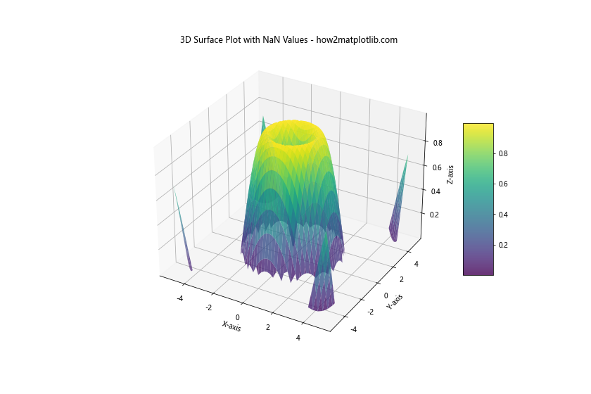
This example demonstrates how to handle NaN values in your dataset by masking them in the surface plot.

Improving Performance for Large Datasets

When dealing with large datasets, 3D surface plotting can become slow. Here are some techniques to improve performance:

import numpy as np
import matplotlib.pyplot as plt
from mpl_toolkits.mplot3d import Axes3D

# Generate a large dataset
x = np.linspace(-10, 10, 1000)
y = np.linspace(-10, 10, 1000)
X, Y = np.meshgrid(x, y)
Z = np.sin(np.sqrt(X**2 + Y**2))

# Create the plot
fig = plt.figure(figsize=(12, 8))
ax = fig.add_subplot(111, projection='3d')

# Plot the surface with optimized settings
surf = ax.plot_surface(X, Y, Z, cmap='viridis',
                       rstride=10, cstride=10,  # Increase stride for better performance
                       linewidth=0, antialiased=False)

# Customize the plot
ax.set_xlabel('X-axis')
ax.set_ylabel('Y-axis')
ax.set_zlabel('Z-axis')
ax.set_title('Optimized 3D Surface Plot for Large Dataset - how2matplotlib.com')

# Add a color bar
fig.colorbar(surf, shrink=0.5, aspect=5)

plt.show()

Output:

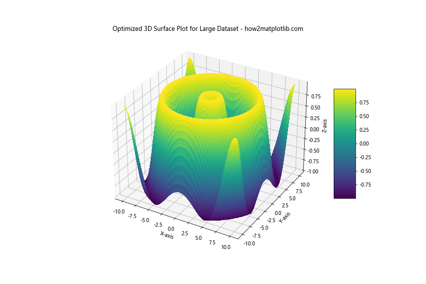
This example shows how to use stride and disable antialiasing to improve performance when plotting large datasets.

Advanced Applications of 3D Surface Plotting in Python using Matplotlib

3D surface plotting in Python using Matplotlib has numerous advanced applications across various fields. Let's explore some interesting use cases:

Visualizing Mathematical Functions

3D surface plots are excellent for visualizing complex mathematical functions:

import numpy as np
import matplotlib.pyplot as plt
from mpl_toolkits.mplot3d import Axes3D

# Generate data
x = np.linspace(-5, 5, 100)
y = np.linspace(-5, 5, 100)
X, Y = np.meshgrid(x, y)
Z = np.sin(X) * np.cos(Y) * np.exp(-np.sqrt(X**2 + Y**2) / 10)

# Create the plot
fig = plt.figure(figsize=(12, 8))
ax = fig.add_subplot(111, projection='3d')

# Plot the surface
surf = ax.plot_surface(X, Y, Z, cmap='coolwarm')

# Customize the plot
ax.set_xlabel('X-axis')
ax.set_ylabel('Y-axis')
ax.set_zlabel('Z-axis')
ax.set_title('3D Visualization of a Complex Function - how2matplotlib.com')

# Add a color bar
fig.colorbar(surf, shrink=0.5, aspect=5)

plt.show()

Output:

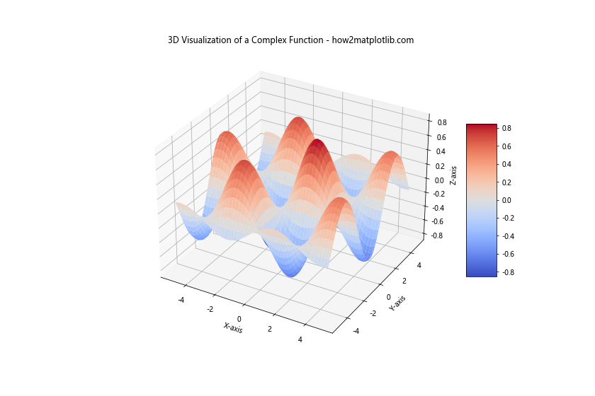
This example visualizes a complex mathematical function using a 3D surface plot.

Representing Geographical Data

3D surface plots can be used to represent geographical data, such as terrain elevation:

import numpy as np
import matplotlib.pyplot as plt
from mpl_toolkits.mplot3d import Axes3D

# Generate sample terrain data
x = np.linspace(0, 10, 100)
y = np.linspace(0, 10, 100)
X, Y = np.meshgrid(x, y)
Z = 2 * np.sin(X) + 3 * np.cos(Y) + np.random.random(X.shape) * 0.5

# Create the plot
fig = plt.figure(figsize=(12, 8))
ax = fig.add_subplot(111, projection='3d')

# Plot the surface
surf = ax.plot_surface(X, Y, Z, cmap='terrain')

# Customize the plot
ax.set_xlabel('Longitude')
ax.set_ylabel('Latitude')
ax.set_zlabel('Elevation')
ax.set_title('3D Terrain Visualization - how2matplotlib.com')

# Add a color bar
fig.colorbar(surf, shrink=0.5, aspect=5, label='Elevation')

plt.show()

Output:

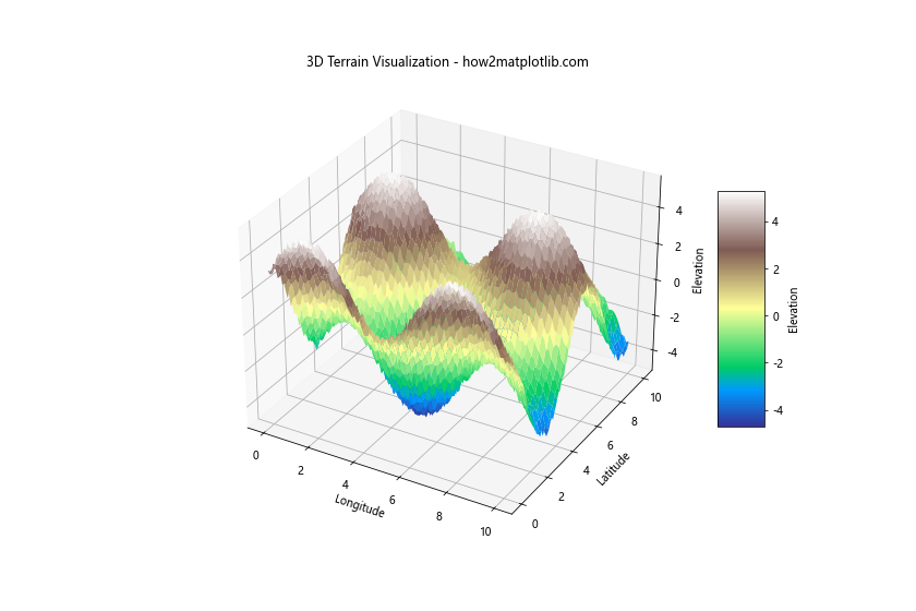
This example demonstrates how to use 3D surface plotting to visualize terrain data.

Conclusion

3D surface plotting in Python using Matplotlib is a powerful tool for visualizing three-dimensional data. Throughout this article, we've explored various techniques, from basic plot creation to advanced customization and optimization. We've covered topics such as color mapping, combining multiple datasets, handling large datasets, and addressing common challenges.

By mastering these techniques, you can create informative and visually appealing 3D surface plots for a wide range of applications, from mathematical visualization to geographical data representation. Remember to experiment with different settings and combinations to find the best way to represent your specific data.